*Corresponding author. phone: +353 1896 1034
Experimental
Validation
of
a
CFD
Methodology
for
Transitional
Flow
Heat
Transfer
Characteristics
of
a
Steady
Impinging
Jet
Sajad Alimohammadi
*[email protected] Trinity College Dublin
Dept. Mechanical and Manufacturing Engineering,
Dublin, Ireland
Darina B. Murray
[email protected] Trinity College Dublin
Dept. Mechanical and Manufacturing Engineering,
Dublin, Ireland
Tim Persoons
[email protected] Trinity College Dublin
Dept. Mechanical and Manufacturing Engineering,
Dublin, Ireland
Abstract
This paper presents a computational fluid dynamics (CFD) methodology to accurately predict the
heat transfer characteristics of an unconfined steady impinging air jet in the transitional flow regime,
impinging on a planar constant-temperature surface. The CFD methodology is validated using
detailed experimental measurements of the local surface heat transfer coefficient. The numerical
model employs a transitional turbulence model which captures the laminar-turbulent transition in the
wall jet which precisely predicts the intensity and extent of the secondary peak in the radial Nusselt
number distribution. The paper proposes a computationally low-cost turbulence model which yields
the most accurate results for a wide range of operating and geometrical conditions. A detailed analysis
of the effect of mesh grid size and properties, inflow conditions, turbulence model, and turbulent
Prandtl number Prt is presented. The numerical uncertainty is quantified by the grid convergence
index (GCI) method. In the range of Reynolds number 6,000 ≤ Re ≤ 14,000 and nozzle-to-surface
distance 1 ≤ H/D≤ 6, the model is in excellent agreement with the experimental data. For the case of
H/D =1 and Re = 14,000, the maximum deviations are 5%, 3% and 2% in terms of local,
area-averaged and stagnation point Nusselt numbers, respectively. Experimental and numerical
correlations are presented for the stagnation point Nusselt number.
Sajad Alimohammadi 2 HT-14-1049
Axisymmetric impinging jet; Local Nusselt number; Numerical modelling; Transitional flow;Shear stress transport; CFD; Experimental Validation
Nomenclature
D nozzle pipe inner diameter, m Tu local turbulence intensity, %
H nozzle-to-impingement surface spacing, m tpipe nozzle pipe wall thickness, m
Nu local Nusselt number x, r axial and radial coordinate (main flow), m
L nozzle length, m y+ non-dimensional distance from the wall
Pr Prandtl number Greek letters
Prt turbulent Prandtl Number A, A absolute and relative uncertainty on quantity A q local convective heat flux, W/m2 density of fluid, kg/m3
Re Reynolds number kinematic viscosity of fluid, m2/s
T local surface temperature, K Subscripts
Tref fluid temperature in jet nozzle, K 0 stagnation point
1
Introduction
Jet impingement is widely used in applications for high heat flux cooling like gas turbine blades
and high-density electronic equipment, so its heat transfer performance has been the subject of many
studies both numerically and experimentally in the last decades, [1-9]. Some studies have
experimentally examined the heat transfer to steady impinging jets issuing from a long pipe nozzle
[1-3] showing that the heat transfer rates are very sensitive to alterations in flow conditions (e.g., velocity
and/or turbulence profile), [4-5]. Viskanta [4], Jambunathan et al. [5] and Persoons et al. [9] have
presented comprehensive overviews of stagnation Nusselt number correlations for a steady impinging
jet on a flat surface. The reported differences between empirical heat transfer correlations are due to
variations in the nozzle geometry and the heat transfer performance enhancement by intensified
velocity gradients and fluctuations. The temporal nature of both the fluid flow and heat transfer of
impinging air jets has been experimentally investigated by O’Donovan and Murray [6]; their results
show that the evolution of vortices with distance from the jet exit has an influence on the magnitude
of heat transfer coefficient along the wall. In another study [7], the same authors have shown that at
low nozzle-to-target ratios (H ≤ 2D), secondary peaks in the radial heat transfer distributions are due
Sajad Alimohammadi 3 HT-14-1049
Various numerical investigations have been performed to study the heat transfer coefficientdistributions of impinging jet flows. A number of numerical studies have qualitatively predicted the
main flow features and heat transfer trends; however the results for local heat transfer distributions do
not consistently produce acceptable quantitative agreement with experiments [10-12]. Furthermore,
there are few studies recommending a reliable computational methodology for transitional jet
impingement. This is the main motivation of the current paper, which uses the established
experimental methodologies of previous studies by the authors [6-7], [9] for validation. As described
by Caggese et al. [12], the inlet turbulence intensity has a strong effect on the heat transfer coefficient
distribution, so the inlet turbulence profile must be chosen appropriately in order to fit the numerical
model with experimental data. As will be described in section 2.1, the profiles of velocity and
turbulence intensity exiting the nozzle are mapped from a separate model for the long inlet nozzle
pipe to make the inlet boundary conditions more realistic.
In computational fluid dynamics, turbulence modelling coupled with appropriate near-wall
treatment of grids is critical for the achievement of accurate flow and heat transfer predictions in
impinging jet flows. There is no clear consensus in the literature on the most robust turbulence model
which yields the best results for a wide range of operating and geometrical conditions. Although some
recent studies using the large eddy simulation (LES) approach have proposed some enhancements in
the accuracy of CFD results comparing to experiments [13-15], the methods are not computationally
efficient enough for a typical industrial design and engineering environment. Thus, performance
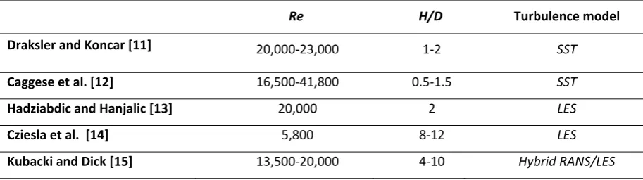
evaluation of computationally efficient turbulence models is a crucial objective for this paper. Table
1 presents an overview of the main parameter ranges and turbulence models used in some selected
numerical studies from the literature. Different CFD models have been used, for a range of Re andH/D values.
In addition, when the simulation domain contains laminar, transitional and turbulent flows at the
same time in different regions, the laminar-turbulent boundary layer transition should be modelled
Sajad Alimohammadi 4 HT-14-1049
the domain [12], this paper employs a transition turbulence model called the Gamma-Theta model[16-18]. This model is based on two transport equations for intermittency and the transition
momentum thickness Reynolds number, which determine the state of the boundary layer. The model
becomes more useful in wall-bounded flows, in which the wall shear stress or the surface heat transfer
rate are of interest. It is designed to predict the location and extent of laminar to turbulent flow
transition which in turn significantly affects the heat transfer coefficient distribution. For impinging
jet heat transfer at low values of nozzle-to-surface ratio (H ≤ 2D [6]), the local increase in wall-normal
velocity fluctuations due to the transition of the wall jet flow from the laminar to turbulent mode
coincides with a secondary peak in the heat transfer coefficient distribution along the wall (see also
Colucci and Viskanta [19]). A recent study by Caggese et al. [12] on circular jet impingement shows
that although numerical modelling can accurately predict the main heat transfer characteristics in the
stagnation zone, it is more difficult to accurately predict this secondary peak.
The current paper aims to establish and verify a robust RANS (Reynolds-averaged Navier-Stokes)
computational fluid dynamics (CFD) methodology to accurately predict the local heat transfer
coefficient for a circular steady impinging jet, using our own detailed experimental measurements for
validation. The goal is to capture the transition to turbulence in the wall jet, ensure the model is valid
in a wide range of operational and geometrical parameters, while keeping the computational cost low.
This study is the first step towards a robust numerical methodology for unsteady impinging flows
such as synthetic or pulsating jets ([9], [20-22]).
2
Numerical
Methodology
For the numerical simulation of jet impingement, the commercial tool ANSYS CFX 14 is
employed. Attention is focused on the near-wall region since it is the most important for convective
heat transfer. Some previous studies on heat transfer to impinging jets only qualitatively predict the
flow physics, with a limited degree of quantitative accuracy for the solution of the energy equation
Sajad Alimohammadi 5 HT-14-1049
accuracy of heat transfer simulations by validating the results via comparison with experimental localheat transfer coefficient data (see Sections 3, 4 and 5).
2.1
Computational Domain: Geometry and Boundary Conditions
Figure 1 displays the three-dimensional axisymmetric computational domain and boundary
conditions used in the simulation of an unconfined round jet impinging on a flat plate. The dimensions
are identical to that of the experimental setup used for validation (see Section 3.1). Considering the
axisymmetric nature of the flow, only a wedge section of the cylindrical domain (with one node in the
circumferential direction) is simulated. An assumption of axisymmetric flow in the domain provides a
good approximation while saving time to achieve a satisfactory convergence (Alimohammadi et al.
[23]), as verified by the comparison of CFD to experimental results presented in sections 4 and 5. The
computational domain extends far enough from the area of interest (up to a radial distance of 16D
from the jet centerline) to prevent outlet boundary effects on the results.
The boundary conditions applied to the domain are shown in Fig 1. Periodic boundary conditions
are applied in the circumferential direction. The velocity profile at the nozzle exit is calculated using a
separate simulation for a long nozzle pipe and mapped from the nozzle exit to the domain inlet. The
spatially and time-averaged velocity in the nozzle is set to match the Reynolds number (based on the
diameter D = 13 mmand the mean nozzle velocity) used in the experiments. The turbulence intensity
at the domain inlet is also determined by means of the same mapping procedure of profiles obtained
for the turbulent kinetic energy from a separate simulation. However, it should be noted that the
turbulence intensity value at the nozzle inlet, which was not measured in the experiments, remains
unknown; the procedure to estimate the averaged turbulence intensity at the nozzle pipe inlet is
described in section 4.4. At the radial outlet and unconfined top boundaries of the domain, an opening
boundary condition with a constant temperature of 25 °C and zero relative pressure is used to allow
the flow to leave and re-enter the domain, thereby enabling potential flow re-circulation. The planar
heated wall surface at the bottom of the domain is set to a constant temperature of 60 °C, in agreement
Sajad Alimohammadi 6 HT-14-1049
2.2
Mesh Generation
The generated mesh is designed to resolve the important flow features as a function of the main
parameters (e.g., Re and H/D), using suitable methods such as grid refinement inside the wall
boundary layer. The mesh topology is generated based on the structured approach with a hexahedral
mesh to maintain the orthogonality in the domain; afterwards, it is refined and adapted iteratively in
regions with large velocity, pressure, temperature and turbulence gradients in order to attain a stable
solution. To have a computationally efficient model in low-gradient regions a coarse mesh scheme is
applied, resulting in better control on the physical distance of the first grid point from the wall (y+).
The adequate value of near-wall cell thickness is ensured by keeping the y+ below unity for the
near-wall cells. Additionally, at least ten nodes are applied inside the viscous laminar sub-layer within a
small distance from the wall (in the order of 10-6×D for the present problem). The final grid is
generated to have a larger concentration of nodes close to the impingement wall and the jet mixing
region. Section 4.1 shows the details of five different mesh sizes used for the grid independency study
and their effect on heat transfer results.
2.3
Fluid Properties
Fluid compressibility is negligible in the current problem since the local Mach number does not
exceed 0.05. However since temperature differences up to 35 °C may occur in the domain, a moderate
change in air properties can be expected. A linear property table is employed to calculate the density,
viscosity and thermal conductivity for the range of 25 °C to 60 °C in the domain, to include the effect
of compressibility and changing fluid properties. As a result, the difference between the heat transfer
results extracted from incompressible and compressible models for the applicable range of Re
numbers in this study (between 6000 and 14,000) is calculated to be less than 1%.
2.4
Turbulence modelling and governing equations
As observed in impinging jet flow experiments, both laminar and turbulent flow occurs
simultaneously in different regions. For laminar flow, the numerical solution of the momentum and
Sajad Alimohammadi 7 HT-14-1049
turbulent or transitional flows, a turbulence model is required. Turbulence strongly affects theimportant global features of the flow, so the accurate and reliable prediction of turbulent flow
phenomena is essential.
The decision about the appropriate model for simulations of turbulence in the domain is based on
the flow physics and computational requirements depending on the generated grid and accuracy. Due
to the boundary layer separation, a wall function is not an appropriate method to resolve the boundary
layer [13]. Instead, directly resolving the boundary layer can provide accurate results. One of the
major considerations is generating a near-wall mesh which is fine enough to resolve the laminar part
of the boundary layer (viscous sub-layer) over a very small distance from the wall. The RANS
turbulence models are broadly used in practical modelling for suitable accuracy and efficiency. The
RANS turbulence models evaluated in the present study are: k-, RNG k-, k-, and SST with and
without a transition model. Section 4.5 describes the effect of the different turbulence models on the
results and the procedure for selection of an appropriate turbulence model in comparison with
experimental data.
The CFD simulations are performed based on the well-known conservation laws for
incompressible flow, namely continuity, momentum and energy equations, plus the appropriate
turbulence equations according to the final selected turbulence model (SST, as will be described in
section 4.5) as a closure [24]. In addition, the present study employs an accurate and realizable
laminar-turbulent transition model called Gamma-Theta model (-Re). This model employs new
empirical correlations developed by Langtry and Menter [16-18], which have been broadly validated
to work with the SST turbulence model.
2.5
Solution Approach
Second order discretization schemes produce more accurate results for heat transfer, yet are less
stable in convergence compared to first order schemes, especially for the energy equation which is
very important for this study. To improve the convergence a multi-step approach is used: firstly, the
Sajad Alimohammadi 8 HT-14-1049
discretization scheme. When the solution meets the convergence criteria of 10-6 for all the equations,the next step of solution starts with a blend of 1st and 2nd order discretization schemes based on the
same convergence criteria, initialized by the results of the previous step; the blend factor is
successively increased from 0 to 1 in order to ensure a full 2nd order scheme at the final step of
simulation.
3
Experimental
Methodology
3.1
Facility and Instrumentation
The validation experiments were performed on an existing impinging jet test facility [6-7], [9].
The geometry is identical to the numerical model shown in Fig. 1. An air jet issues from a nozzle
consisting of a smooth brass pipe with inner diameter D = 13mm and length L = 32D, with a sharp
edged exit, shown schematically in Fig. 2. The pipe length exceeds the hydraulic development length
by about 50% for 6000 Re 14,000. The air flow to the nozzle pipe (a) at a temperature of
approximately 25 °C is supplied by the building air compressor and dehumidification system, via a
pressure regulator (c) and a mass flow controller (b) (MKS 1579A, 0-300 standard liter/min,
combined uncertainty of 3 standard liter/min). The uncertainty in the Reynolds number is determined
as Re = Re/Re [(M/M)2 + (D/D)2]1/2 where M represents the uncertainty in the mass flow rate and
D 0.25mm is the uncertainty in the nozzle diameter. The resulting uncertainty is Re 3-6% for the
investigated range based on a 95% confidence level. For steady flow, the turbulence intensity at the
nozzle exit is below 8.5% of the mean velocity [6].
The heated impingement surface (d) consists of a flat copper plate (425 × 550 mm2, 5 mm thick).
Electrical power is supplied by a DC voltage source to a 1.1 mm thick silicone rubber mat with
embedded wire heaters, glued with thermally conductive adhesive to the underside of the copper
plate. The plate assembly is insulated underneath the heater mat. For typical jet Reynolds numbers,
the representative Biot number equals 0.0013 for the copper plate. The plate approximates a constant
Sajad Alimohammadi 9 HT-14-1049
earlier studies [6]. The system is operated at a fixed surface temperature of 60 C and an ambienttemperature of about 25 C, identical to the CFD simulations.
The local convective heat transfer coefficient is defined as h (= Nuk/D) = q/(TTref) where q is
the local convective heat flux and T is the local surface temperature. Since the flow velocity remains
well below the speed of sound in these tests (Ma < 0.05), the reference temperature Tref is taken as the
jet temperature recorded with a T-type thermocouple mounted in the air supply line upstream of the
pipe nozzle. The uncertainty in the reference and surface temperature is T < 0.1K, based on a 95%
confidence level.
The local convective heat flux q is measured with a factory-calibrated RdF Micro-FoilTM
differential thermopile heat flux sensor (e), which measures the temperature difference across a
well-defined thermal barrier. The manufacturer's calibration coefficient for the heat flux sensor
(0.093V/(W/m2)) is within 3% of the values obtained from a calibration experiment for the stagnation
point Nusselt number in an impinging steady jet issuing from a long pipe nozzle (length = 80D) with a
fully developed velocity profile [3]. For the experimental conditions encountered in this study, the
radiation heat loss from the sensor accounts for about 3-6% of the convection heat flux near the
stagnation point, up to a maximum of about 15% at r/D 4. For the stagnation point, this effect is
intrinsically contained in the heat flux sensor calibration, which is performed at the same surface and
ambient temperature. The resulting uncertainty in the Nusselt number Nu = Nu/Nu [(q/q)2 +
2(T/(T Tref))2]1/2 equals about 6% based on a 95% confidence level, with a spatial resolution of
about 1 mm in the radial direction [6]. The experimental uncertainties are shown as an error band
and/or within the figure caption in the results.
3.2
Experimental Results
Shadlesky [8] used laminar flow theory to derive a lower bound for the stagnation heat transfer
rate to an impinging steady jet with a uniform nozzle velocity profile, Nu0 = 0.5856Re0.5Pr0.4. This
theoretical relationship (represented by the thin solid line in Fig. 3) is valid for approximately H/D <
Sajad Alimohammadi 10 HT-14-1049
stagnation point, Nu0/(Re0.5Pr0.4) 01/2. Since the gradient is steeper for a non-uniform velocityprofile, Nu0/(Re0.5Pr0.4) = 0.5856 can be considered a lower bound for the stagnation point heat
transfer rate to an impinging pipe jet. Figure 3 includes experimental data from other researchers for
stagnation point heat transfer from impinging jet flows from long smooth pipe nozzles. Lytle and
Webb [1] used a pipe of 78D length (0.1 H/D 1, 3600 Re 27600), as Lee and Lee [2] (2 H/D
10, 5000 Re 30,000). Katti and Prabhu [3] used a pipe of 83D long (0.5 H/D 8, 12,000 Re
28,000).
The hollow markers in Fig. 3 represent the current experiments for a steady impinging pipe jet at
H/D = 1, 2, 3, 4, 6 and Re = 6000 (), 10,000 () and 14,000 (). The thick solid line represents a
least squares fitted power law correlation as:
Nu0 = 0.799Re0.5Pr0.4(H/D)0.0436 (R2 = 0.42) (1)
The Nu0 values are at the lower end of those obtained in the other pipe flow studies, which may be
attributed to a lower turbulence level or the shorter pipe length (L = 32D compared to 78-83D) [1-3],
[6], [8].
4
CFD
Validation
and
Sensitivity
Analysis
The following sections present a comprehensive sensitivity analysis of the most influential
methods and parameters in the numerical modelling. Each section discusses an individual aspect of
the CFD methodology using the experimental data for validation. For the sake of clarity, only the
comparisons to the experimental data for Re = 6,000 and H/D = 1 are presented. In all subsequent
figures, experimental data are represented by hollow markers and numerical results by lines without
markers. Although not shown here, the CFD methodology has been verified for the entire range of
Reynolds number and nozzle-to-surface spacing. The effects of Re and H/D on the heat transfer
coefficient distributions are presented in Section 5.
Sajad Alimohammadi 11 HT-14-1049
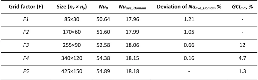
A detailed sensitivity analysis on the grid density is performed to confirm grid independence of thefinal solution. This is performed using 5 sequentially refined grids generated from a baseline mesh F1
(coarse, with 60×20 nodes) by multiplying the cell number by a grid factor (F) of 2 to 5 in all
directions. The details of different grids and their respective heat transfer results, namely the
stagnation point Nusselt number (Nu0) and the area averaged Nusselt number over the whole surface
( ; : ) plus the deviation of the results from the
finest mesh size (i.e. grid factor 5) are shown in Table 2. The Nusselt number is defined as
/ where / and k is the thermal conductivity of the fluid.
According to Table 2, for the grid factor 4, the deviation of Nuave_Domain values from the reference grid
factor is almost negligible. The radial distribution of Nusselt number for different mesh sizes is shown
in Fig. 4(a). The results associated with F4 and F5 almost coincide, except for a minor difference (less
than 1%) in the stagnation region with r/D < 1. A more rigorous numerical uncertainty analysis is also
performed using the method recommended by ASME Journal of Fluids Engineering [25]. The grid
convergence index (GCI) method, performed using three different sets of grids, represents the
discretization error in the solution which is indicated by an error band on the numerical results: Fig.
4(b) shows the local calculated GCI error band for Nusselt number distribution using the grid F4; the
global order of accuracy for grid F4 is 0.9 as oscillatory convergence occurs at 14% of the grid points
in Fig. 4(b). The GCI distribution has some peaks in the region of 1 < r/D < 2 (Fig. 4(b)). The
maximum numerical uncertainty (GCImax) for different grids is also shown in Table 2, indicating that
solutions are within the asymptotic range of convergence. Thus the grid factor 4, with a reasonably
low GCI according to
Table 2, provides an acceptable level of accuracy, and as a compromise between accuracy and
computational time, it is not necessary to employ a finer grid than F4. The selected resolution (F4,with 340 and 120 nodes in and directions, respectively, for H/D = 1) is kept constant through all
Sajad Alimohammadi 12 HT-14-1049
To determine the minimum required vertical distance to the unconfined far-field top boundary,different distances from the heated plate, where Hadd = 0-10D were simulated (see Fig. 1).
For H/D = 1 as the main experimental case, a distance of 3 from the impingement wall has the
closest agreement with experimental data. A further increase no longer affects the Nusselt number
distribution. Gao and Ewing [26] have studied the influence of confinement on the heat transfer to a
round turbulent impinging jet. Their results show that the differences in heat transfer between a
confined and an unconfined jet are negligible for H/D≥ 2, in which case it is possible to impose either
a confined or an unconfined boundary.
4.2
Discretization Scheme
Employing a higher order discretization scheme for the convection term in the conservation
equations is known to increase the simulation accuracy for impinging jet problems ([13]). Although
for the sake of brevity the results are not shown here, a successive enhancement of the discretization
scheme from first order to second order (described in section 2.5) improves the calculated Nusselt
number results compared to the experimental values. The 2nd order scheme resolves the domain to
capture the second peak in Nusselt number distribution in the radial direction. The first order scheme
is inconsistent with the experimental data for the region with r/D < 2, which is mainly attributed to
unstable convergence of the transition equations.
4.3
Inlet Velocity Profile
The heat transfer rate strongly depends on the inlet conditions such as the velocity profile and
turbulence intensity. Figure 5 compares the heat transfer results obtained for different velocity profiles
at the nozzle exit. The fully developed velocity profile is characterized by a higher flow momentum in
the center of the jet compared to the uniform flow, thereby leading to a steeper radial velocity gradient
in the stagnation zone, which Shadlesky [8] has shown to be linked to higher stagnation Nusselt
number. In the present study, the fully developed velocity profile produces a local Nusselt number
distribution in the stagnation region with a maximum deviation of 3% from the experimental data. By
Sajad Alimohammadi 13 HT-14-1049
distribution exhibits a significant deviation from measured data, especially in the stagnation andtransition regions up to r/D = 2 where the uniform and developing profiles under-predict the radial
Nusselt number distribution.
Figure 6 provides a better understanding by comparing the radial distribution of normalized
turbulent kinetic energy in the near-wall region (here: 0.01D from the wall, inside the momentum
boundary layer) for different inlet velocity profiles. The heat transfer coefficient is closely related to
the turbulence intensity and radial velocity gradient. As shown in Fig. 6(a), the turbulent kinetic
energy in the region r/D < 2 is lower for a uniform nozzle exit profile which helps to explain the
Nusselt number deviation from experimental data. For the fully developed profile, the location of the
peak turbulence intensity reasonably matches the secondary peak in the Nusselt number distribution,
corresponding to the laminar-to-turbulent transition. This agrees with the findings of O’Donovan and
Murray [6] and Colucci and Viskanta [19].
The radial velocity gradient in the near-wall region is shown in Fig. 6(b). The jet flow with the
fully developed velocity profile exhibits the steepest radial velocity gradient accompanied by a strong
radial acceleration. The subsequent abrupt deceleration of the wall jet flow coincides with the laminar
to turbulent transition, which is reflected in the secondary Nusselt number peak in Fig. 5. The further
radial development of the wall jet (r/D > 2) shows a monotonic reduction of Nusselt number (Fig. 5)
and a decaying negative velocity gradient (Fig. 6(b)) as the flow spreads out radially.
4.4
Inlet Turbulence Intensity
Consideration should be given to the correct estimation of the turbulence intensity at the nozzle
inlet (Fig. 1). As described in section 5, this is performed using a separate simulation for a long nozzle
pipe, and turbulence intensity profiles are mapped from the nozzle exit to the domain inlet of the main
simulation. The variation in turbulence intensity at the nozzle inlet affects the turbulence intensity
profile at the nozzle exit, and consequently the surface heat transfer, especially at low H/D. Figure
7(a) shows the effect of the nozzle inlet turbulence intensity on the Nusselt number distribution. High
Sajad Alimohammadi 14 HT-14-1049
seen in Fig. 7(a), different turbulence levels mainly affect the intensity and location of the secondarypeak in the Nusselt number distribution. This is known as the transition region (1 < r/D < 2). Except
the low turbulence case (Tu = 1%), the different values from Tu = 2% to 4% produce approximately
the same heat transfer results in the stagnation region (r/D < 1) and developing wall jet region (r/D >
2). Upon comparison with the experimental data, a turbulence intensity of Tu = 3% is selected as the
final value for further numerical investigation of this case. As described by Viskanta [4] and
Jambunathan et al. [5], the inlet turbulence intensity does not have a significant impact for larger
values of H/D where the turbulence created in the shear layer becomes dominant.
4.5
Turbulence Model
As described in section 2.3, the turbulence models evaluated in the present study are: k-, RNG
k-, k-, SST with and without transition model. Figure 7(b) shows the effect of the turbulence model
on the simulation results, with the corresponding experimental data included as markers. The k-,
RNG k- and k- models fail to predict the correct trend of the Nusselt number distribution.
Generally, the k- model is not ideal for the prediction of separation, swirling flows, and flows with
strong streamline curvatures. The k- model works well for the outer region (r/D > 2) but is
unreliable for r/D < 2 where it considerably over-predicts the experimental Nusselt number. For flows
containing recirculation zones, the Shear Stress Transport (SST) model is a better turbulence model,
to be used without additional damping function. One advantage of the SST model is the near-wall
treatment for flow computations at low values of turbulent Reynolds number in the viscous sub-layer.
The SST formulation also switches to the k- behavior in fully turbulent flow fields and thus avoids
the common k- problem where the model is excessively sensitive to the inlet free stream turbulence
properties [13]. A comparison of the different turbulence models for a numerical study of jet
impingement heat transfer has been performed by Zuckerman and Lior [27]. Large errors (up to 60%)
were reported in estimated Nusselt number distributions for most versions of k-, k- and Reynolds
stress models. The authors recommend the SST model for its low computational cost when secondary
Sajad Alimohammadi 15 HT-14-1049
the v2f model with a moderate computational cost, and large eddy simulation (LES) and directnumerical simulation (DNS) with high computational costs. Therefore, the SST model is chosen
coupled with a complementary transition model, as a compromise between low computational cost
and reliably capturing the laminar-to-turbulent transition which is characteristic for these impinging
jet flows.
A critical point in the present study is the correct modelling of the laminar-to-turbulent boundary
layer transition which occurs in the wall jet flow, and directly affects the heat transfer results.
According to Fig. 7(b), the selected transition model coupled with the SST formulation (section 2.4)
accurately predicts the intensity, position and extent of the secondary peak in the radial Nusselt
number distribution. This is the only model which shows a satisfactory agreement with the
experimental data, while the SST without transition model fails to capture the secondary peak. The
current study complements the recent findings of Caggese et al. [12], confirming that the primary
factor in achieving accurate results is the choice of turbulence model, rather than the other
investigated parameters.
4.6
Turbulent Prandtl Number
The turbulent Prandtl Number Prt is the ratio of eddy diffusivities for momentum and heat
transfer. The value of Prt in the near-wall region becomes very important in the prediction of turbulent
heat transfer, since it directly affects heat diffusion. Reynolds [28] reports that the most common way
of relating variations of time-averaged velocity and temperature across a turbulent shear layer is
through the introduction of uniform values for the turbulent Prandtl number. He also suggests values
of Prt = 0.7 for round jets and Prt = 0.5 for other shear flows (e.g., mixing layers, plane jets, and
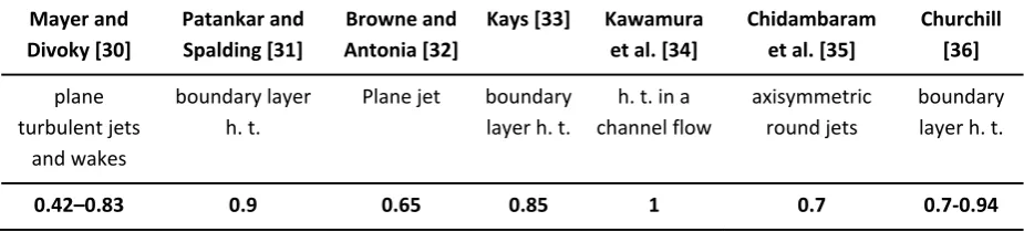
wakes). There have been many discussions in the literature about the parameters that affect the
turbulent Prandtl number in the boundary layer, resulting in quite a lot of semi-empirical correlations
which show the combined dependence of Prt on Reynolds number, molecular Prandtl number and
non-dimensional distance from the wall, , , ([28-36]). Antonia and Kim [29] have
evaluated Prt in turbulent wall shear flows, confirming that Prt tends to a constant value irrespective
Sajad Alimohammadi 16 HT-14-1049
results for Prt from different studies, for the configurations used in the present study. The range ofvalues for Prt shown in Table 3 suggests that the correct value may be different from the default of 0.9
in the Ansys CFX software. The appropriate value for the present case is calculated by comparison of
experimental and numerical results, as shown in Fig. 7(c). Values ranging from 0.7 to 0.8 generate
roughly the same results, except for a minor difference beyond the transition region (Fig. 7(c)). To
accurately capture the intensity and location of the secondary peak in the Nu number distribution, a
value of Prt= 0.7 is chosen here which agrees well with values suggested by the other studies in Table
3. However, it is worth mentioning that a value of Pr = 0.9provides a slightly better prediction of the
area-averaged Nusselt number over the whole region (0 < r/D < 6).
5
Numerical
Results
and
Discussion
5.1
Effect of Reynolds Number
The heat transfer to the impinging jet strongly depends on the Reynolds number. Figure 8
compares the numerical and experimental radial Nusselt number data for Reynolds numbers of 6000,
10,000 and 14,000 for H/D = 1. The nozzle inlet turbulence intensity to ensure best agreement with
the experimental data is Tu = 3% for Re = 6000, Tu = 2% for Re = 10,000 and Tu = 1.5% for 14,000.
Apart from the nozzle inlet turbulence intensity, all other numerical parameters are maintained as
described in Section 4. As shown in Fig. 8, the data for different Reynolds numbers are in acceptable
agreement with the experiments, exhibiting a maximum deviation of 5%, 3% and 2% for Re = 14,000
in terms of local (Nu), area-averaged (Nuave-domain) and stagnation point (Nu0) Nusselt numbers,
respectively. However even for this case the model correctly predicts the heat transfer for r/D < 1,
with the main deviation in the transition region (1 < r/D < 2). Nevertheless the trend is correctly
predicted. This deviation is partly due to the elongation of the potential core at larger Reynolds
number which corresponds to higher jet exit velocities, and partly because of the numerical and
experimental uncertainties which increase with Reynolds number in the transition region.
Sajad Alimohammadi 17 HT-14-1049
As described in section 4.1, the computational mesh size has been kept the same for all theprevious sections, because the domain remained unchanged. The required mesh size to resolve the
flow field and heat transfer in the boundary layer is unique for each nozzle-to-surface distance, and a
distinct mesh is generated for each H/D value according to the procedure in section 4.1.
The position of the secondary Nusselt number peak is a function of both Re and H/D, and both the
experimental and numerical results in Fig. 9 confirm this. O’Donovan and Murray [6] report that for
higher values of H/D the shear layer penetrates to the stagnation point, resulting in a diminished
velocity and increased turbulence intensity at the centerline. In this case the turbulence created in the
shear layer becomes dominant. As shown in Fig. 9, the influence of the inlet conditions becomes
negligible. For the case of H/D = 2, the secondary peaks in numerical predictions are visible with
some degree of deviation in the transition region. This can mainly be attributed to the slight increase
in numerical uncertainty which occurs in the region 1 < r/D < 2 (see section 4.1). This is the reason
for the deviation of the results in the same region for larger values of H/D as well. Also, at larger
values of H/D the axial velocity of the jet in the region up to r/D < 1 is smaller and does not cause the
same wall jet flow development as for small H/D values. Conclusively, the profile does not have an
evident secondary peak in the Nusselt number distribution due to a more uniform turbulence
distribution level, as shown in Figs. 9(c) and (d) for H/D = 4 and 6, respectively.
As with the experimental results (Eq. (1)), two least squares fitted power law correlations of the
stagnation point Nusselt number is derived from the numerical results:
Nu0 = 0.784Re0.5Pr0.4(H/D) 0.064 (R2 = 0.978) (2)
Nu0 = 0.663Re0.518Pr0.4(H/D) 0.064 (R2 = 0.978) (3)
Eq. (2) is based on the assumption of a fixed value for the power of Re number (here 0.5, see Shadleskey [8]), while Eq. (3) uses a least-square fitted value for the power of Re number.
Sajad Alimohammadi 18 HT-14-1049
The performance evaluation of computationally efficient turbulence models shows that withrealistic configurations of boundary conditions, computational domain, fluid properties and solution
approach, numerical modelling is able to accurately predict the local heat transfer coefficient for a
circular steady impinging jet.
The results for the SST turbulence model coupled with Gamma-Theta Transition model, as a
computationally low cost model, show improvements in accurate prediction of the position, intensity
and extent of the secondary peak in the local Nusselt number distribution, as determined from a
comparison with detailed experimental measurements for validation.
Furthermore, by iteratively adapting the grid density in the near-wall region, the large velocity,
temperature and turbulence quantities gradients in the momentum and thermal boundary layers are
well captured. Correlations based on the experimental and numerical heat transfer coefficient data are
generated for the stagnation point Nusselt number for a wide range of operating conditions,
incorporating the effect of Reynolds number (6000 Re 14,000), nozzle-to-surface distance (1
H/D 6) in the standard formulation Nu0 = a.Re0.5Pr0.4(H/D)nwith a = 0.799 and n = 0.0436 for the
experiments and a = 0.784 and n = 0.064 for the numerical model (see Equations (1) and (2)).
The turbulent Prandtl numberin the near-wall region has proven an important parameter in the
prediction of turbulent heat transfer since its value directly affects the level of heat diffusion. Here, to
most accurately capture the intensity and location of the secondary peak in the Nusselt number
distribution, a turbulent Prandtl number value Prt = 0.7 is proposed for the simulations, which is in
line with the values suggested by other studies (see Table 3). However, a value of Prt = 0.9 would
yield slightly more accurate results in terms of the overall area-averaged Nusseltnumber.
By accurately reproducing the experimental boundary conditions in the numerical model, the
simulated Nusselt number distributions in the stagnation region deviate less than 3% from the
experimental results. For the entire range of Reynolds numbers, a maximum deviation of 5% is found
with the experimental local Nusselt numbers, for the case of Re = 14,000. The location of the
Sajad Alimohammadi 19 HT-14-1049
affected significantly by the inlet turbulence intensity for larger values of H/D where the turbulencecreated in the shear layer becomes dominant. The position of the secondary Nusselt number peak
varies consistently with Re and H/D, both in the experiments and numerical results.
The effect of Reynolds number and nozzle-to-surface spacingshows that the computational model
is robust enough for a wide range of geometrical and operational conditions. This provides an
encouraging starting point to extending this numerical methodology towards unsteady impingement
flows such as synthetic or pulsating jets [9], [20]-[22].
Acknowledgements
This work has been partly funded by Science Foundation Ireland (SFI), grant 09-RFP-ENM2151.
References
[1]. Lytle D., and Webb B. W., 1994, “Air-jet impingement heat-transfer at low nozzle plate spacings,” International Journal of Heat and Mass Transfer, 37 (12), pp. 1687–1697.
[2]. Lee J., and Lee S. S., 1999, “Stagnation region heat transfer of a turbulent axisymmetric jet impingement,” Experimental Heat Transfer, 12 (2), pp.137–156.
[3]. Katti V., and Prabhu S. V., 2008, “Experimental study and theoretical analysis of local heat transfer distribution between smooth flat surface and impinging air jet from a circular straight pipe nozzle,” International Journal of Heat and Mass Transfer, 51 (17-18), pp. 4480–4495.
[4]. Viskanta R., 1993, “Heat transfer to impinging isothermal gas and flame jets,” Experimental Thermal and Fluid Science, 6 (2), pp. 111–134.
[5]. Jambunathan K., Lai E., Moss M. A., and Button B. L., 1992, “A review of heat-transfer data for single circular jet impingement,” International Journal of Heat and Fluid Flow, 13 (2), pp. 106–115.
[6]. O’Donovan T. S., and Murray D. B., 2007, “Jet impingement heat transfer – Part I: Mean and root-mean-square heat transfer and velocity distributions,” International Journal of Heat and Mass Transfer, 50, pp.
3291–3301.
[7]. O’Donovan T. S., and Murray D. B., 2007, “Jet impingement heat transfer – Part II: A temporal investigation of heat transfer and local fluid velocities,” International Journal of Heat and Mass Transfer, 50, pp.
3302–3314.
[8]. Shadlesky P. S., 1983, “Jet impingement to a plane surface,” AIAA Journal, 21(8), pp. 1214–1215.
[9]. Persoons T., McGuinn A., and Murray D. B., 2011, “A general correlation for the stagnation point Nusselt number of an axisymmetric impinging synthetic jet,” International Journal of Heat and Mass Transfer,
Sajad Alimohammadi 20 HT-14-1049
[10]. Wang T., Dhanasekaran T. S., 2010, “Calibration of a Computational Model to Predict Mist/Steam Impinging Jets Cooling With an Application to Gas Turbine Blades”, ASME Journal of Heat Transfer, 132, pp.122201:1-11.
[11]. Draksler M., and Koncar B., 2009, “A numerical investigation on a submerged, axis-symmetric jet,” Proceedings of the International Conference Nuclear Energy for New Europe 2009, Slovenia, pp. 822.1-9. [12]. Caggese O., Gnaegi G., Hannema G., Terzis A., and Ott P., 2013, “Experimental and numerical investigation of a fully confined impingement round jet,” International Journal of Heat and Mass Transfer, 65,
pp. 873–882.
[13]. Hadziabdic M., and Hanjalic K., 2008, “Vortical structures and heat transfer in a round impinging jet,” Journal of Fluid Mechanics, 596, pp. 221–260.
[14]. Cziesla T., Biswas G., Chattopadhyay H., Mitra N. K., 2001, “Large-eddy simulation of flow and heat transfer in an impinging slot jet,” International Journal of Heat and Fluid Flow, 22 (5), pp. 500–508.
[15]. Kubacki S., Dick E., 2010, “Simulation of plane impinging jets with k– based hybrid RANS/LES models,” International Journal of Heat and Fluid Flow, 31 (5), pp. 862–878.
[16]. Langtry R. B., and Menter F. R., 2005, “Transition Modelling for General CFD Applications in Aeronautics,” 43rd AIAA Aerospace Sciences Meeting and Exhibit 2005, Reno, Nevada, pp. 522.1-14.
[17]. Menter F. R., Langtry R. B., Likki S. R., Suzen Y. B., Huang P. G., and Voelker S., 2006, “A Correlation-based Transition Model Using Local Variables Part 1 – Model Formulation,” ASME Journal of Turbomachinery, 128 (3), pp. 413-422.
[18]. Langtry R. B., 2006, “A Correlation-based Transition Model Using Local Variables for Unstructured Parallelized CFD Codes, PhD thesis,” Institute of Thermal Turbomachinery and Machinery Laboratory, University of Stuttgart.
[19]. Colucci D. W., and Viskanta R., 1996, “Effect of nozzle geometry on local convective heat transfer to a confined impinging air jet,” Experimental Thermal and Fluid Science, 13 (1), pp. 71-80.
[20]. Persoons T., Balgazin K., Brown K., and Murray D. B., 2013, “Scaling of Convective Heat Transfer Enhancement due to Flow Pulsation in an Axisymmetric Impinging Jet,” ASME Journal of Heat Transfer, 135
(11), pp. 111012:1-10.
[21]. Valiorgue P., Persoons T., McGuinn A., and Murray D. B., 2009, “Heat transfer mechanisms in an impinging synthetic jet for a small jet-to-surface spacing,” Experimental Thermal and Fluid Science, 33 (4), pp.
597–603.
[22]. Alimohammadi S., Persoons T., and Murray D. B., 2014, “A numerical-experimental study of heat transfer enhancement using unconfined steady and pulsating turbulent air jet impingement,” Proc. 15th International Heat Transfer Conference 2014, Kyoto, Japan, IHTC15-8765 (accepted; in press).
[23]. Alimohammadi S., Persoons T., Murray D. B., Tehrani M. S., Farhanieh B., and Koehler J., 2013, “A Validated Numerical-Experimental Design Methodology for a Movable Supersonic Ejector Compressor for Waste-Heat Recovery,” ASME Journal of Thermal Science and Engineering Applications, 6 (2), pp. 021001:1-10.
Sajad Alimohammadi 21 HT-14-1049
[25]. Celik I.B., Ghia U., Roache P.J., Freitas C.J., Coleman H., and Raad P.E., 2008, “Procedure for estimation and reporting of uncertainty due to discretization in CFD applications,” Journal Fluids Engineering,130 (7), pp. 07800-1.
[26]. Gao N., and Ewing D., 2006, “Investigation of the effect of confinement on the heat transfer to round impinging jets exiting a long pipe,” International Journal of Heat and Fluid Flow, 27, pp. 33–41.
[27]. Zuckerman N., and Lior N., 2006, “Jet impingement heat transfer: physics, correlations, and numerical modelling,” Advances in Heat Transfer, 39, pp. 565-631.
[28]. Reynolds A. J., 1976, “The Variation of Turbulent Prandtl and Schmidt Numbers in Wakes and Jets,” International Journal of Heat and Mass Transfer, 19, pp. 757-764.
[29]. Antonia R. A., and Kim J., 1991, “Turbulent Prandtl number in the near-wall region of a turbulent channel flow,” International Journal of Heat and Mass Transfer, 34 (7), pp. 1905-1908.
[30]. Mayer E., and Divoky D., 1966, “Correlation of intermittency with preferential transport of heat and chemical species in turbulent shear flows,” AIAA, 4 (11), pp. 1995–2000.
[31]. Patankar S. V., and Spalding D. B., 1967, “Heat and Mass Transfer in Boundary Layers,” Morgan Grampian, London.
[32]. Browne L. W. B., and Antonia R. A., 1983, “Measurements of Turbulent Prandtl Number in a Plane Jet,” ASME Journal of Heat Transfer, 105 (3), pp. 663-665.
[33]. Kays W.M., 1994, “Turbulent Prandtl number - where are we?,” ASME Journal of Heat Transfer, 116
(2) pp. 284-295.
[34]. Kawamura H., Abe H., and Matsuo Y., 1999, “DNS of turbulent heat transfer in channel flow with respect to Reynolds and Prandtl number effects,” International Journal of Heat and Fluid Flow, 20, pp. 196-207.
[35]. Chidambaram N., Dash S.M., and Kenzakowski D.C., 2001, “Scalar variance transport in the turbulence modelling of propulsive jets,” J. Propul. Power, 17, pp. 79–84.
Sajad Alimohammadi 22 HT-14-1049
List of Table CaptionsTable 1. Overview of parameter ranges and turbulence models used in selected numerical studies
Table 2. Details of different grids and their heat transfer results (Nu0 and Nuave_Domain) with deviation
of Nuave_Domain (%) from grid F5 and maximum uncertainties (GCImax %) for grid independency study
Sajad Alimohammadi 23 HT-14-1049
List of Figure CaptionsFigure 1. Computational domain and boundary conditions used in the simulation of the unconfined axisymmetric impinging jet
Figure 2. Schematic diagram of the experimental setup; (a) pipe nozzle, (b) mass flow meter, (c) pressure reducer valve, (d) instrumented isothermally heated plate, (e) embedded heat flux sensor, and (f) data acquisition unit and computer
Figure 3. Heat transfer coefficient at the stagnation point of a steady impinging jet plotted as Nu0/(Re0.5Pr0.4) as a
function of nozzle-to-surface spacing H/D
Figure 4(a). Radial distribution of Nusselt number for different mesh sizes, F1 to F5, listed in Table 1 (Re = 6,000, H/D = 1); (b). Local distribution of numerical uncertainty (GCI(%)) as error band on the selected mesh size for simulation (F4)
Figure 5. Comparison of radial distribution of Nusselt number for different inlet velocity profiles to experimental data (Re = 6,000, H/D = 1; error bars display exp. uncertainty)
Figure 6. Radial distribution of (a) normalized turbulence kinetic energy and (b) radial velocity gradient (s-1)
near the wall (at 0.01D) for different inlet velocity profiles (Re = 6,000, H/D = 1)
Figure 7. Comparison of radial distribution of Nusselt number for different (a) inlet turbulence intensities (%), (b) turbulence models and (c) turbulent Prandtl numbers to experimental data (Re = 6,000, H/D = 1; Exp. uncertainty = 6%)
Figure 8. Comparison of radial distribution of Nusselt number for different Reynolds numbers to experimental data (H/D = 1; Re = 6,000, 10,000 and 14,000; error bars display exp. uncertainty)
Sajad Alimohammadi 24 HT-14-1049
Table 1Re H/D Turbulence model
Draksler and Koncar [11] 20,000‐23,000 1‐2 SST
Caggese et al. [12] 16,500‐41,800 0.5‐1.5 SST
Hadziabdic and Hanjalic [13] 20,000 2 LES
Cziesla et al. [14] 5,800 8‐12 LES
Sajad Alimohammadi 25 HT-14-1049
Table 2Grid factor (F) Size (nx × ny) Nu0 Nuave_Domain Deviation of Nuave_Domain % GCImax %
F1 85×30 50.64 17.96 1.21 ‐
F2 170×60 51.60 17.99 1.05 ‐
F3 255×90 52.58 18.06 0.66 12
F4 340×120 54.38 18.15 0.16 4.7
Sajad Alimohammadi 26 HT-14-1049
Table 3Mayer and
Divoky [30]
Patankar and
Spalding [31]
Browne and
Antonia [32]
Kays [33] Kawamura
et al. [34]
Chidambaram
et al. [35]
Churchill
[36]
plane turbulent jets
and wakes
boundary layer h. t.
Plane jet boundary
layer h. t.
h. t. in a channel flow
axisymmetric round jets
boundary layer h. t.
![6 (1 Methylethyl) 12 phenyl 5,6,7,12 tetrahydrodibenz[c,f][1,5]azasilocine](data:image/gif;base64,R0lGODlhAQABAIAAAP///wAAACH5BAEAAAAALAAAAAABAAEAAAICRAEAOw==)