Abstract—Instability in a power system may be manifested
in many ways depending on the system configuration and operating mode. Voltage instability in power distribution systems could lead to voltage collapse and thus power blackouts or abnormally low voltages. It is required to know the strength of the buses to improve the voltage stability of the system. This paper analyzes the performance of different voltage stability indices and its enhancement by placing optimal location of Distributed generation (DG). This work proposes analytical expressions for finding optimal size and power factor of distributed generation (DG) units. DG units are sized to achieve the highest loss reduction in distribution networks. The large deployement of distributed generation (DG) sources in distribution network can be an efficient solution to overcome power system technical problems and economical challenges. The method has been tested in 16-bus and 33-bus distribution systems.
Index Terms—Distributed generation, Voltage stability, and voltage stability indices.
I. INTRODUCTION
Recently a top priority is given to develop a reliable, sustainable, environment friendly as well as low-cost electrical energy supply. This includes a sensible energy mix and improvements in efficiency of energy generation, transmission and consumption[1]. As a number of events that have been brought to the vulnerability of the current centralized electrical energy supply infrastructure, such as terrorist threats, natural disasters, geopolitical disruptions, ageing of a highly complex infrastructure, climate change and regulatory and economic risks, DG appears to be one of the key answers for different problems[2]. In the distribution system, the electrical power supply will be transferred from a vertical one to a horizontal system. In the traditional system the electric power industry has been driven by a paradigm where most of the electricity is generated in large power plants, sent to the consumption areas through HVtransmission lines, and delivered to the consumers through a passive distribution infrastructure that involves HV, MV and LV networks. In this paradigm power
Manuscript received March 5, 2016;. Comparison of voltage stability indices and its enhancement using Distributed Generation Kumaraswamy Research scholar JNTUH Hyderabad (e-mail:[email protected] ) S.Tarakalyani professor and HoD department of EEE JNTUH , Hyderabad.( e-mail:[email protected])
B. Venkata prasanth professor & HoD, department of EEE QIS institute of technology ongole.( e-mail:[email protected])
.
flows only in one direction from the power station to the network and to the consumer.
The DG term is used to describe small distribution system close to the point of consumption. Such generators may be owned by a utility or more likely by a customer who may use the entire portion or perhaps all of it to the local utility combustion turbine generators, internal combustion engines and generators, photovoltaic panels, and fuel cells. Solar thermal conversion, stirling engines, are considered as DG. When the penetration of DG is high, the generated power of DG units not power flow in the distribution network consequence, the connection of DG to the grid may different technical issues, e.g. voltage profiles quality, stability etc..[3] In spite of the benefits of utilizing DG units within of the system efficiency and the improvements in the technical and operational challenge units into MV distribution networks are needed. Moreover, in more details with respect to the generation types. Optimization of the MV distribution networks with a large penetration of DG is Also needed therefore the utilities can get more benefits[4].
Distributed generation can be considered as taking power to the load. Distributed generator promises to generate electricity with high efficiency and low pollution. Unlike large central power plants, Distributed generator can be installed at or near the load. Distributed generator ratings range from 5 kW up to 100 MW. Maintenance cost for embedded generation such as fuel cells and photovoltaic’s is quite low because of the lack of moving parts. Several recent developments have optimistic the entry of power generation and energy storage at the distribution level. Some of the major ones are listed below. With expanded choice, customers are demanding customized power supplies to suit their needs.
Advent of several technologies with reduced environmental impacts and high conversion efficiencies.
Advent of efficient and cost-effective power electronic interfaces to improve power quality and reliability.
Ability to effectively control a number of components and subsystems using state-of-the-art computers to manage loads, demands, power flows, and customer requirements.
Several Distributed generation technologies are under various stages of development. They include micro turbines, photovoltaic systems (PV), wind energy conversion systems (WECS), gas turbines, gas-fired IC engines, diesel engines, and fuel cell systems. At present, wind energy has become the most competitive among all renewable energy technologies. Integration of DG into an existing utility can
Comparison of Voltage Stability Indices and its
Enhancement Using Distributed Generation
result in several benefits. These benefits include line loss reduction, reduced environmental impacts, peak shaving, increased overall energy efficiency, relieved transmission and distribution congestion, voltage support.
The Distributed Generation (DG) has created a challenge and an chance for developing various novel technologies in power generation. The work discusses the primary factors that have lead to an increasing interest in DG. DG reduces line losses, increases system voltage profile.
II.RADIALDISTRIBUTIONNETWORK
The load flow of a power system provides the steady state solution through which various parameters like currents, voltages, losses etc can be calculated. It is a very important and fundamental tool for the analysis of any power system and is used in the operational as well as planning stages. Many methods such as Gauss-Seidel, Newton-Raphson are well reported to carry out the load flow of transmission system. The use of these methods for distribution system may not be advantageous because they are mostly based on the general meshed topology of a typical transmission system where as most distribution systems have a radial or tree structure. Further distribution system posses high R/X ratio, which cause the distribution systems to be ill conditioned for conventional load flow methods.
Some other inherent characteristics of electric distribution systems are
• Radial or weakly meshed structure. • Multiphase and unbalanced operation. • Unbalanced distributed load.
• Extremely large number of branches and nodes. • Wide-ranging resistance and reactance values.
The efficiency of the optimization problem of distribution system depends on the load flow algorithm because load flow solution has to run for many times. Therefore, the load flow solution of distribution system should have robust and time efficient characteristics. A method which can find the load flow solution of radial distribution system directly by using topological characteristic of distribution network [1, 2] is used. In this method, the formulation of time consuming Jacobian matrix or admittance matrix, which are required in the conventional methods, is avoided. This method is explained in brief.
Mathematical Model
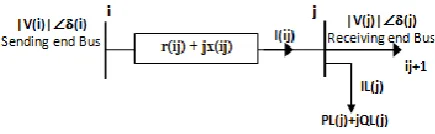
In fig 1, |V(i)|(i) and |V(j)|(j) are the voltage magnitudes and phase angles of two buses i and j respectively and current flowing through the line ij is I(ij). The substation voltage is assumed to be (1+j0) p.u.
[image:2.595.60.278.679.746.2]
Fig. 1 Equivalent circuit model of RDS of a typical branch ij
(a) Branch Currents
From the electric equivalent of a feeder branch shown in Fig. 1.1, we can write the load current and charging current equations (1.1) and (1.2) respectively for bus j [25].
* *
) j ( V
) j ( jQL ) j ( PL )
j ( V
) j ( SL
IL(j)
j = 2, 3, …nd --- (2.1)
IC(j)y(j)V(j) j = 2, 3, …nd……….(2.2)
Current through the branch ij is equal to the sum of the all buses load currents and charging currents beyond the line ij by including the line ij receiving end bus load current and charging current Thus, the line current following through the line ij can be computed using eqn. (2.3):
branch ij the after availablek allthebuses branch
ij the after availablek allthebuses
) k ( IC )
k ( IL
I(ij)
ij = 1, 2, 3…. br--- (2.3)
where br is the number of branches (b) Bus Voltages
Therefore, the generalized equation of receiving end voltage, sending end voltage, line current and line
impedance is V(j)V(i)-I(ij)Z(ij)
ij = 1, 2, 3…. br………. (2.4)
where
Z(ij)r(ij) jx(ij)Impedance of branch ij = 1, 2, 3…. br (2.5) where Impedance of branch ij (c) Real and Reactive Power Losses
The real and reactive power loss of each branch ij is given by:
r(ij) I(ij) (ij)
Ploss 2
ij = 1, 2, 3…. br
(2.6)
x(ij) I(ij) (ij)
Qloss 2
ij = 1, 2, 3…. Br--- (2.7)
(d) Proposed Solution Technique
convergence criterion. Here 0.00001p.u. is taken as tolerance value.
(e) Process of buses identification beyond a particular branch
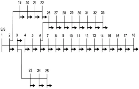
[image:3.595.84.286.145.266.2]Consider the single line diagram of 16-bus radial distribution system which is shown in Fig. 2 Buses 1,2 and 3 are considered as substations, and remaining as load buses.
Fig. 2 Single line diagram of 16-node Radial Distribution system
[image:3.595.53.284.349.496.2]Consider the single line diagram of 33-bus radial distribution system which is shown in Fig.3 Bus 1, are considered as substation, and remaining as load buses.
Fig. 3 Single line diagram of 33-node Radial Distribution system
Consider the single line diagram of 33-bus radial distribution system which is shown in Fig.2.2 Bus 1, are considered as substation, and remaining as load buses.
III. VOLTAGESTABILITY
Voltage stability states that voltage stability is the ability of a power system to maintain steady acceptable voltage at all buses in the system under normal operating conditions and after being subjected to a disturbance. A system enters a state of voltage instability when a disturbance, increase in load demand or change in system conditions, causes a progressive and uncontrollable drop in voltage [5]. Voltage stability depends on the ability to maintain or restore equilibrium between load demand and load supply from the power system.
According to [6], voltage instability stems from the attempt of load dynamics to restore power consumption beyond the capability of the combined transmission and generation system. Instability occurs in the form of a progressive fall or rise of voltages of some buses. A possible outcome of voltage instability is loss of load in an area, or tripping of
transmission lines and other elements by their protective systems.
The main factor causing instability is the inability of the power system to meet the demand for the reactive power. The reactive power can be supplied by generators through transmission networks or compensated directly at load buses by compensators such as shunt capacitors. There are two side effects of reactive power transmission: transmission losses and voltage drops. In response to a disturbance, power consumed by the loads tends to be restored by the action of motor slip adjustment, distribution voltage regulators, tap-changing transformers and thermostats. Therefore, restored loads increase the stress on the high voltage network by increasing the reactive power consumption and causing further voltage reduction [7]. It is judged that a system is voltage unstable if, for at least one bus in the system, the bus voltage magnitude decreases as the reactive power injection in the same bus is increased [5]. The term voltage collapse refers to the process by which the sequence of events accompanying voltage instability leads to a blackout or abnormally low voltages in a significant part of the power system [7]. In complex practical power systems, many factors
many factors contribute to the
process of system collapse because of voltage
instability: strength of transmission system,
power-transfer levels, load characteristics, generator
reactive power capability limits and characteristics
of reactive power compensating devices [5].
VOLTAGE STABILIYY INDICES:
In voltage stability analysis, it is useful to assess voltage stability of power systems by means of voltage stability indices (VSI), scalar magnitudes that can be monitored as system parameters change. Operators can use these indices to know how close the system is to voltage collapse in an intuitive manner and react accordingly.
a)Bus voltage computation indices:
L-INDEX:
The L index was first described in [8] and it is based on a hybrid representation of the transmission system with the following set of equations:
l L U LG L
G G GL GG G
V
I
Z
F
I
H
I
V
K
Y
V
---(3.1)Where
𝑉𝐿, 𝐼𝐿 are the voltage and current vectors at the load buses 𝑉𝐺, 𝐼𝐺 are the voltage and current vectors at the generator buses
𝑍U,𝐾𝐺𝐿,𝐹𝐿𝐺,𝑌𝐺𝐺 are the sub-matrices of the hybrid matrix H.
Thus, the index can also be expressed in power
terms as following:
exchanged against their currents. This representation can then be used to define a voltage stability indicator at each load bus.
0
2
1
j jj
j ij j
V
S
L
V
Y
V
---(3.2)J j jcorr
S
S
S
---(3.3)ij i
jcorr j
i L ij i i j
Z S
S
V
Z V
---(3.4)The complex term
𝑆
𝑗𝑐o𝑟𝑟 represents the contributionsof the other loads in the system to the index
evaluated at node
j.
When a load bus approaches a collapse point, the
index value is 1. The nodes with the higher value are
considered the weaker buses of the system.
VOLTSGE STABILITY INDEX (VSI):
VSI is defined by mathematical expression,
SI(r)=2VS2−2Vr2− Vr2 -2Vr2(PR+QX)−|Z|2(P2+Q2)-(3.5)b)LINE STABILITY INDICES:
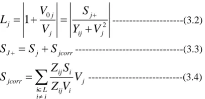
[image:4.595.49.253.97.196.2]
Most of line stability indices are formulated based on the power transmission concept in a single line. A single line in an interconnected network is illustrated in Fig 4.
Fig. 4 Two bus system
Where,
𝑉𝑠 𝑎𝑛𝑑 𝑉𝑟 are the sending end and receiving end voltages, respectively.
𝛿𝑠 𝑎𝑛𝑑 𝛿𝑟 are the phase angle at the sending and receiving buses.
Z is the line impedance. R is the line resistance. X is the line reactance. θ is the line impedance angle.
𝑄𝑟 is the reactive power at the receiving end. 𝑃𝑟 is the active power at the receiving end. (i) Lmn Index
This index proposed in [8] is based on the concept of power flow through a single line and adopting the technique of reducing a power system network into a single line
.
)
6
.
3
...(
1
)]
-sin(
[
4
2
s
r
V
XQ
Lmn
(ii)LQP Index :
This index defined in [9] uses the same concept as in the previous index Lmn. Using the same notation, the proposed index is calculated as following:
4
(
2)(
2 i2 j)...(
3
.
7
)
ii
Q
P
V
X
V
X
LQP
(iii) Fast Voltage Stability Index (FVSI)
This index proposed by [10] stands for Fast Voltage Stability Index (FVSI) and it is also based on the concept of power flow through a single line.
)
8
.
3
...(
4
2 2
s r
V
Q
Z
FVSI
IV: OPTIMAL DG LOCATION AND SIZE FOR LOSS REDUCTION
Due to the increase in power demand, the need for generation of power is steadily increasing. To give uninterrupted service to consumers, it is necessary to increase the penetration of distributed generation into distribution systems. Due to the problems of poor voltage regulation, shortage of transmission capacities and increased environmental concerns, the conventional methods of supplying power could not meet the whole demand. To overcome this, distributed generator (DG) has become the alternative source for power supply[12].
Apart from meeting the energy demand, the optimal location and size of DG units can reduce distribution losses; improve voltage stability and voltage profile. If DG units are improperly allocated and sized, the reverse power flow from larger DG units can lead to higher system losses. Loss minimization is an important factor in planning and operation of DG. Many techniques have been proposed in literature to find the optimal allocation and optimal size of DG.
The exhaustive load flow (ELF) method and an improved analytical (IA) method are used for allocation of DG. Unlike the previous methods, DG is capable of injecting both real and reactive powers. As DG units can supply a portion of total power to loads, the feeder current reduces from the source to the DG location.
a) PROPOSED METHODOLOGY:
The exact power loss equation is given by
...(4.1)1 1
N
i N j
j i j i ij j i j i ij
L PP QQ QP PQ
P
Where
i j
j i
ij ij j i j i
ij
ij
sin
V
V
r
,
cos
V
V
r
i i
V
the complex voltage at the bus ith;ij ij
ij
jx
Z
j i
and
P
P
The active power injections at the ith and jth buses, respectively;j i
and
Q
Q
The reactive power injections at the ith and jth buses, respectively;N the number of buses.
SIZING AT VARIOUS LOCATIONS
Assuming a = (sign) tan(cos-1(PFDG)), the reactive power output of DG is expressed by eqn. (4.2)
QDGi = aPDGi ... (4.2) in which
sign = +1: DG injecting reactive power; sign = −1: DG consuming reactive power; PFDG is the power factor of DG.
The active and reactive power injected at bus i, where the DG located, are given by eqn. (4.3) and eqn. (4.4), respectively,
Pi = PDGi - PDi ….. (4.3)
Qi = QDGi - QDi = aPDGi - QDi ….(4.4)
The power factor of DG depends on operating conditions and type of DG. When the power factor of DG is given, the optimal size of DG at each bus i for minimizing losses can be found in the following way.
1) Type 1 DG: For Type 1 DG, power factor is at unity, i.e., PFDG = 1, a = 0. The optimal size of DG at each bus i for minimizing losses can be given by equation (4.5)
....(4.5) 11
N i j j j ij j ij Di ii ii DiDGi P Q P Q
P
2) Type 2 DG: Assuming PFDG = 0 and a = ∞, The optimal size of DG at each bus i for minimizing losses is given by reduced equation (4.6).
....(4.6)1
1
N i j j j ij j ij Di ii ii DiDGi Q P Q P
Q
3) Type 3 DG: Assuming 0 < PFDG < 1, sign = +1 and “a” is a constant, the optimal size of DG at each bus i for the minimum loss is given by (4.7) and (4.4), respectively.
) 7 . 4 ...( 2 ii ii i i Di Di ii Di Di ii DGi a aY X Q aP aQ P P 4) Type 4 DG: Assuming 0 < PFDG < 1, sign = −1 and “a” is a constant, the optimal size of DG at each bus i for the minimum loss is given by (4.7) and (4.4), respectively.
OPTIMAL POWER FACTOR:
Consider a simple distribution system with two buses, a source, a load and DG connected through a transmission line as shown in Fig. 5.
Fig.5. Simple distribution system with DG.
The power factor of the single load (PFD2 ) is given by equation (4.8)
The power factor of the single load (PFD2 ) is given by
)
8
.
4
...(
2 2 2 2 2 2 D D D DQ
P
P
PF
It can be proved that at the minimum loss occur when power factor of DG is equal to the power factor of load as given by equation (4.9).
)
9
.
4
...(
2 2 2 2 2 2 2 DG DG DG DG DQ
P
P
PF
PF
In practice, a complex distribution system includes a few sources, many buses, many lines and loads[12-13]. The power factors of loads are different. If each load is supplied by each local DG, at which the power factor of each DG is equal to that of each load, there is no current in the lines. The total line power loss is zero. The transmission lines are also unnecessary. However, that is unrealistic since the capital investment cost for DG is too high. Therefore, the number of installed DGs should be limited.
To find the optimal power factor of DG for a radial complex distribution system, fast and repeated methods are proposed. It is interesting to note that in all the three test systems the
Source PDG2+jQDG2
1 2
Bus 2 V2 2
PD2+jQD2
P12+jQ12
R+jX
Bus 1 V1
optimal power factor of DG (Type 3) placed for loss reduction found to be closer to the power factor of combined load of respective system.
Fast Approach: Power factor of combined total load of the system (PFD ) can be expressed by equation (4.8). In this condition, the total active and reactive power of the load demand are expressed as
ni Di
D
P
P
1(4.10)
ni Di
D
Q
Q
1(4.11)
The “possible minimum” total loss can be achieved if the power factor of DG (PFDG) is quickly selected to be equal to that of the total load (PFD). That can be expressed by equation (4.12).
Repeated Approach: In this method, the optimal power factor is found by calculating power factors of DG (change in a small step of 0.01) near to the power factor of combined load. The sizes and locations of DG at various power factors with respect to losses are identified from equation (4.3). The losses are compared together. The optimal power factor of DG for which the total loss is at minimum is determined.
Di
DG
Q
PF
(4.12)V
RESULTS AND ANALYSIS OF VARIOUS LINE AND BUS STABILITY INDICES:Simulations were run on the 16-buses,33-buses and,69-Buses Radial distribution Test System. The real and reactive power losses obtained through load flow.
The results shown in table 1 are the assorted types of line indices and bus indices.
Lmn, FVSI and LQP are the line indices, where as L-index is the bus indices.
To examine the voltage stability margin the value of various line indices is ≤ 1. If all the line indices are ≤ 1,then the system is secure region(stable) otherwise it is unstable. i,e line indices ≥1.
Fig. 2 shows the single line diagram of 16-bus radial distribution system. Buses 1, 2 and 3 are considered as substations, and remaining as load buses. by observing the results the all the load buses values are less than one so we conclude that all the line and bus indices are stable.
[image:6.595.306.545.83.304.2]Total real power load : 28700.00 kW Total reactive power load : 17300.00 kVAr Total real power loss : 2827.14 kW Total reactive power loss : 3248.25 kVAr Minimum Voltage : 0.83872
Table 1: Comparative Results of various indices for voltage stability analysis-16 bus system
S.No Lmn FVSI LQP L-Index
1 0.0813 0.0813 0.0521 0.0083
2 0.0123 0.0129 0.0084 0.0098
3 0.0332 0.0347 0.0278 0.0066
4 0.018 0.0192 0.0096 0.0062
5 0.157 0.1566 0.0786 0.0157
6 0.0079 0.0088 0.0056 0.0173
7 0.0389 0.0436 0.0218 0.0044
8 0.0227 0.0267 0.0134 0.0025
9 0.059 0.0695 0.0454 0.0156
10 0.0011 0.0011 0.0005 0.0102
11 0.037 0.038 0.0243 0.0119
12 0.0033 0.0034 0.0022 0.0101
[image:6.595.304.545.360.779.2]13 0.0116 0.0121 0.006 0.0101
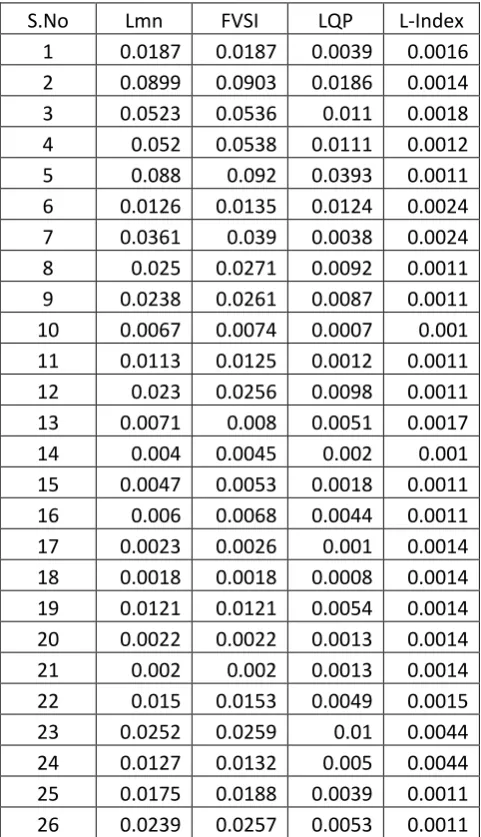
Table 2: Comparative Results of various indices for voltage stability analysis-33 bus system
S.No Lmn FVSI LQP L-Index
1 0.0187 0.0187 0.0039 0.0016
2 0.0899 0.0903 0.0186 0.0014
3 0.0523 0.0536 0.011 0.0018
4 0.052 0.0538 0.0111 0.0012
5 0.088 0.092 0.0393 0.0011
6 0.0126 0.0135 0.0124 0.0024
7 0.0361 0.039 0.0038 0.0024
8 0.025 0.0271 0.0092 0.0011
9 0.0238 0.0261 0.0087 0.0011
10 0.0067 0.0074 0.0007 0.001
11 0.0113 0.0125 0.0012 0.0011
12 0.023 0.0256 0.0098 0.0011
13 0.0071 0.008 0.0051 0.0017
14 0.004 0.0045 0.002 0.001
15 0.0047 0.0053 0.0018 0.0011
16 0.006 0.0068 0.0044 0.0011
17 0.0023 0.0026 0.001 0.0014
18 0.0018 0.0018 0.0008 0.0014
19 0.0121 0.0121 0.0054 0.0014
20 0.0022 0.0022 0.0013 0.0014
21 0.002 0.002 0.0013 0.0014
22 0.015 0.0153 0.0049 0.0015
23 0.0252 0.0259 0.01 0.0044
24 0.0127 0.0132 0.005 0.0044
25 0.0175 0.0188 0.0039 0.0011
27 0.0698 0.0754 0.033 0.0011
28 0.0522 0.0574 0.0248 0.0017
29 0.0375 0.0418 0.0086 0.0055
30 0.0152 0.017 0.0084 0.0019
31 0.0033 0.0037 0.0021 0.0024
32 0.0011 0.0013 0.0009 0.0024
VI. CONCLUSION
This paper analyzes the performance of different voltage stability indices and its enhancement by placing optimal location of Distributed generation (DG). This work proposes analytical expressions for finding optimal size and power factor of distributed generation (DG) units. DG units are sized to achieve the highest loss reduction in distribution networks. The large deployement of distributed generation (DG) sources in distribution network can be an efficient solution to overcome power system technical problems and economical challenges.
References
[1] Acharya N,Mahat P, ithulananthanN,(2006) “An Analytical Approach for DG Allocation in primary Distribution network”, int J. Electric power Energy syst., Vol.28,pp.669-678.
[2] Borges c, Falcao D,(2006) “ optimal , Distributed Generation allocation for reliability , losses ,and voltage improvement”, int J. Electric power Energy syst., Vol.28,pp.413-420.
[3] Hedayati H, Nabaviniaki sa,Akbarimajd a,(2008) “A method for placement of DG units in distribution networks”,IEEE transactions on power delivary ,vol.23, p.p 1620-1628.
[4] Khalesi N, ReZaei N, Haghifam M-R,(2011) “DG Allocation with Application of dynamic programming for loss reduction and reliability improvement”, int J. Electric power Energy syst., Vol.33,pp.288-295.
[5] P. Kundur, Power System Stability and Control. New York: McGraw-Hill, 1994.
[6] T. Van Cutsem and C. Vournas, Voltage Stability of Electric Power Systems. Norwell, MA: Kluwer, 1998.
[7] P. Kundur et al., “Definition and classification of power system stability”, IEEE Transactions on Power Systems, Vol. 19, No. 2, May 2004, pp. 1387-1401. [8] P. Kessel and H. Glavitsch, “Estimating the voltage
stability of a power system”, IEEE Transactions on Power Delivery, Vol.PWRD-1, No.3, July 1986, pp. 346-353.
[9] B. Gao, G.K. Morison and P. Kundur, “Towards the development of a systematic approach for voltage stability assessment of large-scale power systems,” IEEE Transactions on Power Systems, Vol. 11, No. 3, August 1996, pp. 1314.
[10] C. W. Taylor, Power System Voltage Stability. New York: McGraw-Hill, 1994.
[11] F. Karbalaei, H. Soleymani and S. Afsharnia, “A comparison of voltage collapse proximity indicators”, IPEC 2010 Conference Proceedings, 27-29 Oct. 2010, pp. 429-432.
[12] M. E.Baran and F. F.Wu, “Network reconfiguration in distribution systems for loss reduction and load balancing,” IEEE Trans. Power Del., vol. 4, no. 2, pp. 1401–1407, Apr. 1989.