Nonconvex Global Optimization for Latent Variable Models

Nonconvex Global Optimization for Latent-Variable Models

Department of Computer Science Johns Hopkins University, Baltimore, MD

{mrg,jason_}@cs.jhu.edu

Abstract

Many models in NLP involve latent vari-ables, such as unknown parses, tags, or alignments. Finding the optimal model pa-rameters is then usually a difficult noncon-vex optimization problem. The usual prac-tice is to settle forlocaloptimization meth-ods such as EM or gradient ascent. We explore how one might instead search for aglobaloptimum in parameter space, using branch-and-bound. Our method would eventually find the global maxi-mum (up to a user-specified) if run for

long enough, but at any point can return a suboptimal solution together with an up-per bound on the global maximum. As an illustrative case, we study a gener-ative model for dependency parsing. We search for the maximum-likelihood model parameters and corpus parse, subject to posterior constraints. We show how to for-mulate this as a mixed integer quadratic programming problem with nonlinear con-straints. We use the Reformulation Lin-earization Technique to produce convex relaxations during branch-and-bound. Al-though these techniques do not yet pro-vide a practical solution to our instance of this NP-hard problem, they sometimes find better solutions than Viterbi EM with random restarts, in the same time.

1 Introduction

Rich models with latent linguistic variables are popular in computational linguistics, but in gen-eral it is not known how to find their optimal pa-rameters. In this paper, we present some “new” at-tacks for this common optimization setting, drawn from the mathematical programming toolbox.

We focus on the well-studied but unsolved task of unsupervised dependency parsing (i.e.,

depen-∗_{This research was partially funded by the JHU Human} Language Technology Center of Excellence.

-180.2

-231.0 -254.3

-387.1 -287.3 -311.1 -467.5

-298 -342 !5" -0.6 -0.6 "!5

!5" -2 -2 "!5 !3" -0.6 -0.6 "!3

!2" -0.6 -0.6 "!2

Branch-and-bound tree: Incumbent solution:

$ $

M

�

m=1

θmf·m=−400

θ= [−0.1,−0.6,−20,−1.3, . . .] f= [4,0,2,21, . . .]

M �

i=1

θmfm=−400

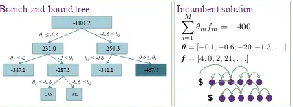
Figure 1: Each node contains a local upper bound for its subspace, computed by a relaxation. The node branches on a single model parameterθm to

partition its subspace. The lower bound, -400, is given by the best solution seen so far, the incum-bent. The upper bound, -298, is the min of all re-maining leaf nodes. The node with a local bound of -467.5 can be pruned because no solution within its subspace could be better than the incumbent.

dency grammar induction). This may be a par-ticularly hard case, but its structure is typical. Many parameter estimation techniques have been attempted, including expectation-maximization (EM) (Klein and Manning, 2004; Spitkovsky et al., 2010a), contrastive estimation (Smith and Eis-ner, 2006; Smith, 2006), Viterbi EM (Spitkovsky et al., 2010b), and variational EM (Naseem et al., 2010; Cohen et al., 2009; Cohen and Smith, 2009). These are alllocal search techniques, which im-prove the parameters by hill-climbing.

The problem with local search is that it gets stuck in local optima. This is evident for gram-mar induction. An algorithm such as EM will find numerous different solutions when randomly ini-tialized to different points (Charniak, 1993; Smith, 2006). A variety of ways to find better local op-tima have been explored, including heuristic ini-tialization of the model parameters (Spitkovsky et al., 2010a), random restarts (Smith, 2006), and annealing (Smith and Eisner, 2006; Smith, 2006). Others have achieved accuracy improve-ments by enforcing linguistically motivated pos-terior constraintson the parameters (Gillenwater et al., 2010; Naseem et al., 2010), such as requir-ing most sentences to have verbs or encouragrequir-ing nouns to be children of verbs or prepositions.

We introduce a method that performs global

search with certificates of -optimality for both the corpus parse and the model parameters. Our search objective is log-likelihood. We can also im-pose posterior constraints on the latent structure.

As we show, maximizing the joint log-likelihood of the parses and the parameters can be formulated as a mathematical program (MP) with a nonconvex quadratic objective and with integer linear and nonlinear constraints. Note that this ob-jective is that of hard (Viterbi) EM—we do not marginalize over the parses as in classical EM.1

To globally optimize the objective function, we employ a branch-and-bound algorithm that searches the continuous space of the model param-eters by branching on individual paramparam-eters (see Figure 1). Thus, our branch-and-bound tree serves to recursively subdivide the global parameter hy-percube. Each node represents a search problem over one of the resulting boxes (i.e., orthotopes).

The crucial step is to prune nodes high in the tree by determining that their boxescannotcontain the global maximum. We compute an upper bound at each node by solving a relaxed maximization problem tailored to its box. If this upper bound is worse than our current best solution, we can prune the node. If not, we split the box again via another branching decision and retry on the two halves.

At each node, our relaxation derives a linear programming problem (LP) that can be efficiently solved by the dual simplex method. First, we lin-early relax the constraints that grammar rule prob-abilities sum to 1—these constraints are nonlin-ear in our parameters, which arelog-probabilities. Second, we linearize the quadratic objective by ap-plying the Reformulation Linearization Technique (RLT) (Sherali and Adams, 1990), a method of forming tight linear relaxations of various types of MPs: thereformulationstep multiplies together pairs of the original linear constraints to generate new quadratic constraints, and then the lineariza-tionstep replaces quadratic terms in the new con-straints with auxiliary variables.

Finally, if the node is not pruned, we search for a better incumbent solution under that node by projecting the solution of the RLT relaxation back onto the feasible region. In the relaxation, the model parameters might sum to slightly more than

1_{This objective might not be a great sacrifice: Spitkovsky} et al. (2010b) present evidence that hard EM can outperform soft EM for grammar induction in a hill-climbing setting. We use it because it is a quadratic objective. However, maximiz-ing it remains NP-hard (Cohen and Smith, 2010).

one and the parses can consist of fractional depen-dency edges. We project in order to compute the true objective and compare with other solutions.

Our results demonstrate that our method can ob-tain higher likelihoods than Viterbi EM with ran-dom restarts. Furthermore, we show how posterior constraints inspired by Gillenwater et al. (2010) and Naseem et al. (2010) can easily be applied in our framework to obtain competitive accuracies using a simple model, the Dependency Model with Valence (Klein and Manning, 2004). We also ob-tain an-optimal solution on a toy dataset.

We caution that the linear relaxations are very loose on larger boxes. Since we have many dimen-sions, the binary branch-and-bound tree may have to grow quite deep before the boxes become small enough to prune. This is why nonconvex quadratic optimization by LP-based branch-and-bound usu-ally fails with more than 80 variables (Burer and Vandenbussche, 2009). Even our smallest (toy) problems have hundreds of variables, so our exper-imental results mainly just illuminate the method’s behavior. Nonetheless, we offer the method as a new tool which, just as for local search, might be combined with other forms of problem-specific guidance to produce more practical results.

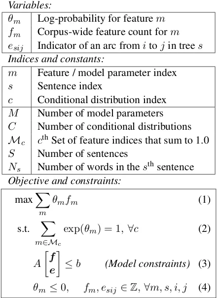
2 The Constrained Optimization Task We begin by describing how for our typical model, the Viterbi EM objective can be formulated as a mixed integer quadratic programming(MIQP) problem withnonlinear constraints(Figure 2).

Other locally normalized log-linear generative models (Berg-Kirkpatrick et al., 2010) would have a similar formulation. In such models, the log-likelihood objective is simply a linear function of the feature counts. However, the objective be-comes quadratic in unsupervised learning, be-cause the feature counts are themselves unknown variables to be optimized. The feature counts are constrained to be derived from the latent variables (e.g., parses), which are unknown discrete struc-tures that must be encoded withintegervariables. The nonlinear constraints ensure that the model parameters are true log-probabilities.

Concretely, (1) specifies the Viterbi EM objec-tive: the total log-probability of the best parse trees under the parametersθ, given by a sum of

log-probabilitiesθmof the individual steps needed

to generate the tree, as encoded by the features

Variables:

θm Log-probability for featurem

fm Corpus-wide feature count form

esij Indicator of an arc fromitojin trees

Indices and constants:

m Feature / model parameter index s Sentence index

c Conditional distribution index M Number of model parameters C Number of conditional distributions

Mc cth Set of feature indices that sum to 1.0

S Number of sentences

Ns Number of words in thesthsentence

Objective and constraints: maxX

m

θmfm (1)

s.t. X

m∈Mc

exp(θm) = 1,∀c (2)

A

f e

≤b (Model constraints) (3)

θm≤0, fm, esij ∈Z,∀m, s, i, j (4)

Figure 2: Viterbi EM as a mathematical program

probabilities are in (2). The linear constraints in (3) will ensure that the arc variables for each sen-tence es encode a valid latent dependency tree,

and that thef variables count up the features of

these trees. The final constraints (4) simply spec-ify the range of possible values for the model pa-rameters and their integer count variables.

Our experiments use the dependency model with valence (DMV) (Klein and Manning, 2004). This generative model defines a joint distribution over the sentences and their dependency trees.

We encode the DMV using integer linear con-straints on the arc variables e and feature counts f. These will constitute the model constraints in (3). The constraints must declaratively specify that the arcs form a valid dependency tree and that the resulting feature values are as defined by the DMV.

Tree Constraints To ensure that our arc vari-ables,es, form a dependency tree, we employ the

same single-commodity flow constraints of Mag-nanti and Wolsey (1994) as adapted by Martins et al. (2009) for parsing. We also use the projectivity constraints of Martins et al. (2009).

The single-commodity flow constraints simul-taneously enforce that each node has exactly one parent, the special root node (position 0) has no

in-coming arcs, and the arcs form a connected graph. For each sentence,s, the variableφsij indicates

the amount of flow traversing the arc fromitojin

sentences. The constraints below specify that the root node emitsNsunits of flow (5), that one unit

of flow is consumed by each each node (6), that the flow is zero on each disabled arc (7), and that the arcs are binary variables (8).

Single-commodity flow (Magnanti & Wolsey, 1994)

Ns

X

j=1

φs0j =Ns,∀j (5)

Ns

X

i=0

φsij− Ns

X

k=1

φsjk = 1,∀j (6)

φsij ≤Nsesij,∀i, j (7)

esij ∈ {0,1},∀i, j (8)

Projectivity is enforced by adding a constraint (9) for each arc ensuring that no edges will cross that arc if it is enabled.Xij is the set of arcs(k, l)

that cross the arc(i, j).

Projectivity (Martins et al., 2009)

X

(k,l)∈Xij

eskl≤Ns(1−esij),∀s, i, j (9)

DMV Feature Counts The DMV generates a dependency tree recursively as follows. First the head word of the sentence is generated, t _∼

Discrete(θroot), where θroot is a subvector of θ.

To generate its children on the left side, we flip a coin to decide whether an adjacent child is gen-erated, d _∼ Bernoulli(θdec.L.0,t). If the coin flip

dcomes upcontinue, we sample the word of that

child ast0 _∼Discrete(θchild.L,t). We continue

gen-erating non-adjacent children in this way, using coin weights θdec.L.≥1,t until the coin comes up stop. We repeat this procedure to generate

chil-dren on therightside, using the model parameters

θdec.R.0,t, θchild.R,t, and θdec.R.≥1,t. For each new

child, we apply this process recursively to gener-ate its descendants.

The feature count variables for the DMV are en-coded in our MP as various sums over the edge variables. We begin with the root/child feature counts. The constraint (10) defines the feature count for model parameter θroot,t as the number

of all enabled arcs connecting the root node to a word of typet, summing over all sentencess. The

constraint in (11) similarly definesfchild.L,t,t0to be

typetto a left child of typet0.Wstis the index set

of tokens in sentencesswith word typet.

DMV root/child feature counts

froot,t= Ns

X

s=1

X

j∈Wst

es0j,∀t (10)

fchild.L,t,t0 =

Ns

X

s=1

X

j<i

δhi∈Wst∧

j∈Wst0

i

esij,∀t, t0 (11)

The decision feature counts require the addi-tion of an auxiliary count variablesfm(si) ∈ Z

in-dicating how many times decision featuremfired

at some position in the corpuss, i. We then need

only add a constraint that the corpus wide fea-ture count is the sum of these token-level feafea-ture countsfm=PSs=1

PNs

i=1f (si)

m ,∀m.

Below we define these auxiliary variables for

1 ≤ s ≤ S and1 ≤ i ≤ Ns. The helper

vari-ablens,i,lcounts the number of enabled arcs to the

left of tokeniin sentences. Lettdenote the word

type of token i in sentences. Constraints (11)

-(16) are defined analogously for theright side fea-ture counts.

DMV decision feature counts

ns,i,l = i−1

X

j=1

esij (12)

ns,i,l/Ns≤f_dec.L.(s,i)_0,t,cont ≤1 (13)

f_dec.L.(s,i)_0,t,stop= 1₋f_dec.L.(s,i)_0,t,cont (14)

f_dec.L.(s,i)_≥1,t,stop =f_dec.L.(s,i)_0,t,cont (15)

f_dec.L.(s,i)_≥1,t,cont =ns,i,l−f_dec.L.(s,i)_0,t,cont (16)

3 A Branch-and-Bound Algorithm The mixed integer quadratic program with nonlin-ear constraints, given in the previous section, max-imizes the nonconvex Viterbi EM objective and is NP-hard to solve (Cohen and Smith, 2010). The standard approach to optimizing this program is local search by the hard (Viterbi) EM algorithm. Yet local search can only provide a lower (pes-simistic) bound on the global maximum.

We propose a branch-and-bound algorithm, which will iteratively tighten both pessimistic and optimistic bounds on the optimal solution. This algorithm may be halted at any time, to obtain the best current solution and a bound on how much better the global optimum could be.

A feasible solution is an assignment to all

the variables—both model parameters and corpus parse—that satisfies all constraints. Our branch-and-bound algorithm maintains anincumbent so-lution: the best known feasible solution according to the objective function. This is updated as better feasible solutions are found.

Our algorithm implicitly defines a search tree in which each node corresponds to a region of model parameter space. Our search procedure begins with only the root node, which represents the full model parameter space. At each node we perform three steps: bounding, projecting, and branching.

In thebounding step, we solve a relaxation of the original problem to provide an upper bound on the objective achievable within that node’s subre-gion. A node is pruned whenLglobal+|Lglobal| ≥

Ulocal, whereLglobalis the incumbent score,Ulocal

is the upper bound for the node, and > 0. This

ensures that its entire subregion will not yield a

-better solution than the current incumbent.

The overall optimistic bound is given by the worst optimistic bound of all current leaf nodes.

The projectingstep, if the node is not pruned, projects the solution of the relaxation back to the feasible region, replacing the current incumbent if this projection provides a better lower bound.

In thebranchingstep, we choose a variableθm

on which to divide. Each of the child nodes re-ceives a lowerθmin_m and upperθmax_m bound forθm.

The child subspaces partition the parent subspace. The search tree is defined by a variable order-ing and the splittorder-ing procedure. We do binary branching on the variableθm with the highest

re-gret, defined as zm − θmfm, where zm is the

auxiliary objective variable we will introduce in

§ 4.2. Since θm is a log-probability, we split its

current range at the midpoint in probability space,

log((expθ_mmin+ expθ_mmax)/2).

We perform best-first search, ordering the nodes by the the optimistic bound of their parent. We also use the LP-guided rule (Martin, 2000; Achter-berg, 2007, section 6.1) to perform depth-first plunges in search of better incumbents.

4 Relaxations

We present successive relaxations to the orig-inal nonconvex mixed integer quadratic program with nonlinear constraints from (1)–(4). First, we show how the nonlinear sum-to-one constraints can be relaxed into linear constraints and tight-ened. Second, we apply a classic approach to bound the nonconvex quadratic objective by a lin-ear concave envelope. Finally, we present our full relaxation based on the Reformulation Lineariza-tion Technique (RLT) (Sherali and Adams, 1990). We solve these LPs by the dual simplex algorithm.

4.1 Relaxing the sum-to-one constraint In this section, we use cutting planes to create a linear relaxation for the sum-to-one constraint (2). When relaxing a constraint, we must ensure that any assignment of the variables that was feasible (i.e. respected the constraints) in the original prob-lem must also be feasible in the relaxation. In most cases, the relaxation is not perfectly tight and so will have an enlarged space of feasible solutions.

We begin by weakening constraint (2) to X

m∈Mc

exp(θm)≤1 (17)

The optimal solution under (17) still satisfies the original equality constraint (2) because of the maximization. We now relax (17) by approx-imating the surface z = P_m∈Mcexp(θm) by

the max ofN lower-bounding linear functions on

R|Mc|. Instead of requiring_z≤1, we only require

each of these lower bounds to be ≤ 1, slightly

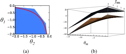
enlarging the feasible space into a convex poly-tope. Figure 3a shows the feasible region con-structed from N=3 linear functions on two

log-probabilitiesθ1, θ2.

Formally, for each c, we define the ith linear

lower bound (i= 1, . . . , N) to be the tangent

hy-perplane at some point_θˆ(i)

c = [ˆθ (i) c,1, . . . ,θˆ

(i) c,|Mc|]∈

R|Mc|, where each coordinate is a log-probability ˆ

θ(i)c,m < 0. We require each of these linear

func-tions to be≤1:

Sum-to-one Relaxation

X

m∈Mc

θm+ 1−θˆ(i)c,m

expθˆ(i)_c,m≤1,∀i, ∀c

(18)

4.2 “Relaxing” the objective

Our true maximization objectiveP_mθmfmin (1)

is a sum of quadratic terms. If the parameters θ

(a)

0 1 2 3 4 fsm

�15 �10 �5

Θm

�60 �40 �20 0 20

(b)

Figure 3: In (a), the area under the curve corre-sponds to those points (θ1, θ2) that satisfy (17)

(z_≤1), with equality (2) achieved along the curve

(z = 1). The shaded area shows the enlarged fea-sible region under the linear relaxation. In (b), the curved lower surface represents a single prod-uct term in the objective. The piecewise-linear up-per surface is its concave envelope (raised by 20 for illustration; in reality they touch).

were fixed, the objective would become linear in the latent features. Although the parameters are not fixed, the branch-and-bound algorithm does box them into a small region, where the quadratic objective is “more linear.”

Since it is easy to maximize a concave function, we will maximize theconcave envelope—the con-cave function that most tightly upper-bounds our objective over the region. This turns out to be piecewise linearand can be maximized with an LP solver. Smaller regions yield tighter bounds.

Each node of the branch-and-bound tree speci-fies a region via bounds constraintsθ_mmin < θm <

θmax_m ,∀m. In addition, we have known bounds f_mmin_≤fm≤fmmax,∀mfor the count variables.

McCormick (1976) described the concave enve-lope for asinglequadratic term subject to bounds constraints (Figure 3b). In our case:

θmfm≤min[fmmaxθm+θminm fm−θminm fmmax,

f_mminθm+θmaxm fm−θmaxm fmmin]

We replace our objectiveP_mθmfmwithPmzm,

where we would like to constrain each auxiliary variable zm to be = θmfm or (equivalently) ≤

θmfm, but instead settle for making it≤the

con-cave envelope—a linear programming problem:

Concave Envelope Objective

maxX

m

zm (19)

s.t.zm≤fmmaxθm+θminm fm−θmminfmmax (20)

4.3 Reformulation Linearization Technique The Reformulation Linearization Technique (RLT)2 _{(Sherali and Adams, 1990) is a method}

of forming tighter relaxations of various types of MPs. The basic method reformulates the problem by adding products of existing constraints. The quadratic terms in the objective and in these new constraints are redefined as auxiliary variables, thereby linearizing the program.

In this section, we will show how the RLT can be applied to our grammar induction problem and contrast it with the concave envelope relaxation presented in section 4.2.

Consider the original MP in equations (1) -(4), with the nonlinear sum-to-one constraints in (2) replaced by our linear constraints proposed in (18). If we remove the integer constraints in (4), the result is a quadratic program withpurely linear constraints. Such problems have the form

maxxTQx (22)

s.t.Ax_≤b (23)

− ∞< Li≤xi ≤Ui <∞,∀i (24)

where the variables are x ∈ Rn_{, A is anm×n}

matrix, andb∈Rm_{, andQis ann×nindefinite}3

matrix. Without loss of generality we assumeQis

symmetric. The application of the RLT here was first considered by Sherali and Tuncbilek (1995).

For convenience of presentation, we repre-sent both the linear inequality constraints and the bounds constraints, under a different parameteri-zation using the matrixGand vectorg.

"

(bi−Aix)≥0, 1≤i≤m

(Uk−xk)≥0, 1≤k≤n

(₋Lk+xk)≥0, 1≤k≤n

#

≡h(gi−Gix)≥0,

1_≤i_≤m+ 2n

i

Thereformulationstep forms all possible products of these linear constraints and then adds them to the original quadratic program.

(gi−Gix)(gj−Gjx)≥0,∀1≤i≤j ≤m+ 2n

In the linearization step, we replace all quadratic terms in the quadratic objective and new quadratic constraints with auxiliary variables:

wij ≡xixj,∀1≤i≤j≤n

2_{The key idea underlying the RLT was originally} intro-duced in Adams and Sherali (1986) for 0-1 quadratic pro-gramming. It has since been extended to various other set-tings; see Sherali and Liberti (2008) for a complete survey.

3_{In the general case, thatQis indefinite causes this} pro-gram to be nonconvex, making this problem NP-hard to solve (Vavasis, 1991; Pardalos, 1991).

This yields the following RLT relaxation:

RLT Relaxation

max X

1≤i≤j≤n

Qijwij (25)

s.t.gigj− n

X

k=1

gjGikxk− n

X

k=1

giGjkxk

+

n

X

k=1 n

X

l=1

GikGjlwkl ≥0,

∀1≤i≤j≤m+ 2n (26)

Notice above that we have omitted the original inequality constraints (23) and bounds (24), be-cause they are fully enforced by the new RLT con-straints (26) from the reformulation step (Sherali and Tuncbilek, 1995). In our experiments, we keep the original constraints and instead explore subsets of the RLT constraints.

If the original QP contains equality constraints of the form Gex = ge, then we can form

con-straints by multiplying this one by each variable

xi. This gives us the following new set of

con-straints, for each equality constraint e: gexi +

Pn

j=1−Gejwij = 0,∀1≤i≤n.

Theoretical Properties The new constraints in eq. (26) will impose the concave envelope con-straints (20)–(21) (Anstreicher, 2009).

The constraints presented above are consid-ered to befirst-level constraints corresponding to the first-level variables wij. However, the same

technique can be applied repeatedly to produce polynomial constraints of higher degree. These higher level constraints/variables have been shown to provide increasingly tighter relaxations (Sher-ali and Adams, 1990) at the cost of a large num-ber of variables and constraints. In the case where

x∈ {0,1}n_{the degree-nRLT constraints will}

re-strict to the convex hull of the feasible solutions (Sherali and Adams, 1990).

4.4 Adding Posterior Constraints

It is a simple extension to impose posterior con-straints within our framework. Here we empha-size constraints that are analogous to the universal linguistic constraints from Naseem et al. (2010). Since we optimize the Viterbi EM objective, we directly constrain the counts in the single corpus parse rather than expected counts from a distribu-tion over parses. LetE be the index set of model

parameters corresponding to edge types from Ta-ble 1 of Naseem et al. (2010), andNsbe the

num-ber of words in the sth sentence. We impose

the constraint that 75% of edges come from _E:

P

m∈Efm ≥0.75PSs=1Ns

.

5 Projections

A pessimistic bound, from the projecting step, will correspond to a feasible but not necessarily opti-mal solution to the original problem. We propose several methods for obtaining pessimistic bounds during the branch-and-bound search, by projecting and improving the solutions found by the relax-ation. A solution to the relaxation may be infea-sible in the original problem for two reasons: the model parameters might not sum to one, and/or the parse may contain fractional edges.

Model Parameters For each set of model pa-rameters Mcthat should sum-to-one, we project

the model parameters onto the Mc −1 simplex

by one of two methods: (1) normalize the infeasi-ble parameters or (2) find the point on the simplex that has minimum Euclidean distance to the infea-sible parameters using the algorithm of Chen and Ye (2011). For both methods, we can optionally apply add-λsmoothing before projecting.

Parses Since we are interested in projecting the fractional parse onto the space of projective span-ning trees, we can simply employ a dynamic pro-gramming parsing algorithm (Eisner and Satta, 1999) where the weight of each edge is given as the fraction of the edge variable.

Only one of these projection techniques is needed. We then either useparsing to fill in the optimal parse trees given the projected model pa-rameters, or usesupervised parameter estimation to fill in the optimal model parameters given the projected parses. These correspond to the Viterbi E step and M step, respectively. We can locally

improve the projected solution by continuing with a few additional iterations of Viterbi EM.

Related models could use very similar projec-tion techniques. Given a relaxed joint soluprojec-tion to the parameters and the latent variables, one must be able to project it to a nearby feasible one, by projecting either the fractional parameters or the fractional latent variables into the feasible space and then solving exactly for the other.

6 Related Work

The goal of this work was to better understand and address the non-convexity of maximum-likelihood training with latent variables, especially parses.

Gimpel and Smith (2012) proposed a concave model for unsupervised dependency parsing us-ing IBM Model 1. This model did not include a tree constraint, but instead initialized EM on the DMV. By contrast, our approach incorporates the tree constraints directly into our convex relaxation and embeds the relaxation in a branch-and-bound algorithm capable of solving the original DMV maximum-likelihood estimation problem.

Spectral learning constitutes a wholly differ-ent family of consistdiffer-ent estimators, which achieve efficiency because they sidestep maximizing the nonconvex likelihood function. Hsu et al. (2009) introduced a spectral learner for a large class of HMMs. For supervised parsing, spectral learn-ing has been used to learn latent variable PCFGs (Cohen et al., 2012) and hidden-state dependency grammars (Luque et al., 2012). Alas, there are not yet any spectral learning methods that recover latent treestructure, as in grammar induction.

Several integer linear programming (ILP) for-mulations of dependency parsing (Riedel and Clarke, 2006; Martins et al., 2009; Riedel et al., 2012) inspired our definition of grammar induc-tion as a MP. Recent work uses branch-and-bound for decoding with non-local features (Qian and Liu, 2013). These differ from our work by treating the model parameters as constants, thereby yield-ing a linear objective.

7 Experiments

We first analyze the behavior of our method on a toy synthetic dataset. Next, we compare various parameter settings for branch-and-bound by esti-mating the total solution time. Finally, we com-pare our search method to Viterbi EM on a small subset of the Penn Treebank.

All our experiments use the DMV for unsuper-vised dependency parsing of part-of-speech (POS) tag sequences. For Viterbi EM we initialize the pa-rameters of the model uniformly, breaking parser ties randomly in the first E-step (Spitkovsky et al., 2010b). This initializer is state-of-the-art for Viterbi EM. We also apply add-one smoothing during each M-step. We use random restarts, and select the model with the highest likelihood.

We add posterior constraints to Viterbi EM’s E-step. First, we run a relaxed linear programming (LP) parser, then project the (possibly fractional) parses back to the feasible region. If the resulting parse does not respect the posterior constraints, we discard it. The posterior constraint in the LP parser is tighter4_{than the one used in the true}

optimiza-tion problem, so the projecoptimiza-tions tends to be feasi-ble under the true (looser) posterior constraints. In our experiments, all but one projection respected the constraints. We solve all LPs with CPLEX.

7.1 Synthetic Data

For our toy example, we generate sentences from a synthetic DMV over three POS tags (Verb, Noun, Adjective) with parameters chosen to favor short sentences with English word order.

In Figure 4 we show that the quality of the root relaxation increases as we approach the full set of RLT constraints. That the number of possible RLT constraints increases quadratically with the length of the corpus poses a serious challenge. For just 20 sentences from this synthetic model, the RLT generates 4,056,498 constraints.

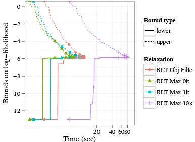
For a single run of branch-and-bound, Figure 5 shows the global upper and lower bounds over time.5 _{We consider five relaxations, each using}

only a subset of the RLT constraints. Max.0k uses only the concave envelope (20)-(21). Max.1k uses the concave envelope and also randomly sam-ples 1,000 other RLT constraints, and so on for Max.10k and Max.100k. Obj.Filter includes all

4_{80%of edges must come from}

Eas opposed to75%. 5_{The initial incumbent solution for branch-and-bound is} obtained by running Viterbi EM with 10 random restarts.

!4

!3

!2

!1

0 ! ! !

!

! !

!

! ! ! !

0.0 0.2 0.4 0.6 0.8 1.0

Proportion of RLT rows included

Upper bound on

log

!

lik

elihood at root

Figure 4: The bound quality at the root improves as the proportion of RLT constraints increases, on 5 synthetic sentences. A random subset of 70%

of the 320,126 possible RLT constraints matches the relaxation quality of the full set. This bound is very tight: the relaxations in Figure 5 solve hun-dreds of nodes before such a bound is achieved.

!12

!10

!8

!6

!4

!2 0

! !

! !

!!!!

! !

! ! !!!!

20 40 6080 Time (sec)

Bounds on log

!

lik

elihood

Bound type lower upper

Relaxation

! _{RLT Obj.Filter}

RLT Max.0k RLT Max.1k

RLT Max.10k

Figure 5: The global upper and lower bounds improve over time for branch-and-bound using different subsets of RLT constraints on 5 syn-thetic sentences. Each solves the problem to

-optimality for=0.01. A point marks every 200

nodes processed. (The time axis is log-scaled.)

constraints with a nonzero coefficient for one of the RLT variables zm from the linearized

ob-jective. The rightmost lines correspond to RLT Max.10k: despite providing the tightest (local) bound at each node, it processed only 110 nodes in the time it tookRLT Max.1kto process 1164.RLT Max.0kachieves the best balance of tight bounds and speed per node.

7.2 Comparing branch-and-bound strategies It is prohibitively expensive to repeatedly run our algorithm to completion with a variety of param-eter settings. Instead, we estimate the size of the branch-and-bound tree and the solution time using a high-variance estimate that is effective for com-parisons (Lobjois and Lemaˆıtre, 1998).

RLT

Re-laxation Avg. msper node # Sam-ples Est. #Nodes Est. #Hours Obj.Filter 63 10000 3.2E+08 4.6E+09 Max.0k 6 10000 1.7E+10 7.8E+10 Max.1k 15 10000 3.5E+08 4.2E+09 Max.10k 161 10000 1.3E+09 3.4E+10 Max.100k 232259 5 1.7E+09 9.7E+13

Table 1: Branch-and-bound node count and com-pletion time estimates. Each standard deviation was close in magnitude to the estimate itself. We ran for 8 hours, stopping at 10,000 samples on 8 synthetic sentences.

can view the branch-and-bound treeTas fixed and

finite in size. We wish to estimate some cost asso-ciated with the tree C(T) = P_{α∈nodes(T)}f(α).

Lettingf(α) = 1estimates the number of nodes;

if f(α) is the time to solve a node, then we

es-timate the total solution time using the Monte Carlo method of Knuth (1975). Table 1 gives these estimates, for the same five RLT relaxations. Obj.Filteryields the smallest estimated tree size.

7.3 Real Data

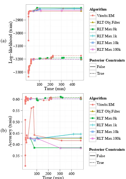
In this section, we compare our global search method to Viterbi EM with random restarts each with or without posterior constraints. We use 200 sentences of no more than 10 tokens from the WSJ portion of the Penn Treebank. We reduce the tree-bank’s gold part-of-speech (POS) tags to a univer-sal set of 12 tags (Petrov et al., 2012) plus a tag for auxiliaries, ignoring punctuation. Each search method is run for 8 hours. We obtain the initial incumbent solution for branch-and-bound by run-ning Viterbi EM for 45 minutes. The average time to solve a node’s relaxation ranges from 3 seconds forRLT Max.0kto 42 seconds forRLT Max.100k. Figure 6a shows the log-likelihood of the in-cumbent solution over time. In our global search method, like Viterbi EM, the posterior constraints lead to lower log-likelihoods. RLT Max.0k finds the highest log-likelihood solution.

Figure 6b compares the unlabeled directed de-pendency accuracyof the incumbent solution. In both global and local search, the posterior con-straints lead to higher accuracies. Viterbi EM with posterior constraints demonstrates the oscil-lation of incumbent accuracy: starting at58.02%

accuracy, it finds several high accuracy solutions early on (61.02%), but quickly abandons them to

increase likelihood, yielding a final accuracy of

60.65%. RLT Max.0k with posterior constraints

obtains the highest overall accuracy of61.09%at (a) !3300 !3200 !3100 !3000 !2900 ! ! ! ! ! ! ! ! ! ! ! !!! ! ! ! !!!!!!!! ! ! !!! ! !! ! ! ! ! !!! !!! ! !!!!!!!!!!!! !

100 200 300 400 Time (min) Log ! lik elihood (train) Algorithm

! _{Viterbi EM}

RLT Obj.Filter RLT Max.0k RLT Max.1k RLT Max.10k RLT Max.100k Posterior Constraints False True (b) 0.35 0.40 0.45 0.50 0.55 0.60 ! ! ! ! ! ! ! ! ! ! ! ! !! ! ! ! ! ! ! ! ! !!! ! ! !_!!! ! ! ! ! ! ! ! !! !! ! ! !!!!!!!!!!!! !

100 200 300 400

Time (min)

Accurac

y (train)

Algorithm

! _{Viterbi EM}

RLT Obj.Filter RLT Max.0k RLT Max.1k RLT Max.10k RLT Max.100k Posterior Constraints False True

Figure 6: Likelihood (a) and accuracy (b) of in-cumbent solution so far, on a small real dataset.

306 min and the highest final accuracy60.73%.

8 Discussion

In principle, our branch-and-bound method can approach-optimal solutions to Viterbi training of

locally normalized generative models, including the NP-hard case of grammar induction with the DMV. The method can also be used with posterior constraints or a regularized objective.

Future work includes algorithmic improve-ments for solving the relaxation and the develop-ment of tighter relaxations. The Dantzig-Wolfe decomposition (Dantzig and Wolfe, 1960) or La-grangian Relaxation (Held and Karp, 1970) might satisfy both of these goals by pushing the inte-ger tree constraints into a subproblem solved by a dynamic programming parser. Recent work on semidefinite relaxations (Anstreicher, 2009) sug-gests they may provide tighter bounds at the ex-pense of greater computation time.

References

Tobias Achterberg. 2007.Constraint integer program-ming. Ph.D. thesis, TU Berlin.

Warren P. Adams and Hanif D. Sherali. 1986. A tight linearization and an algorithm for zero-one quadratic programming problems. Management Science, 32(10):1274–1290, October. ArticleType: research-article / Full publication date: Oct., 1986 / Copyright 1986 INFORMS.

Kurt Anstreicher. 2009. Semidefinite programming versus the reformulation-linearization technique for nonconvex quadratically constrained quadratic pro-gramming. Journal of Global Optimization, 43(2):471–484.

Taylor Berg-Kirkpatrick, Alexandre Bouchard-Cˆot´e, DeNero, John DeNero, and Dan Klein. 2010. Pain-less unsupervised learning with features. InProc. of NAACL, June.

Samuel Burer and Dieter Vandenbussche. 2009. Glob-ally solving box-constrained nonconvex quadratic programs with semidefinite-based finite branch-and-bound. Computational Optimization and Applica-tions, 43(2):181–195.

Olivier Chapelle, Vikas Sindhwani, and S. Sathiya Keerthi. 2007. Branch and bound for semi-supervised support vector machines. In Proc. of NIPS 19, pages 217–224. MIT Press.

E. Charniak. 1993.Statistical language learning. MIT press.

Yunmei Chen and Xiaojing Ye. 2011. Projection onto a simplex. arXiv:1101.6081, January.

Noam Chomsky and Howard Lasnik. 1993. Princi-ples and parameters theory. InSyntax: An Interna-tional Handbook of Contemporary Research. Berlin: de Gruyter.

Shay Cohen and Noah A. Smith. 2009. Shared logis-tic normal distributions for soft parameter tying in unsupervised grammar induction. InProc. of HLT-NAACL, pages 74–82, June.

Shay Cohen and Noah A. Smith. 2010. Viterbi training for PCFGs: Hardness results and competitiveness of uniform initialization. InProc. of ACL, pages 1502– 1511, July.

S. B. Cohen, K. Gimpel, and N. A. Smith. 2009. Lo-gistic normal priors for unsupervised probabilistic grammar induction. InProceedings of NIPS.

Shay B. Cohen, Karl Stratos, Michael Collins, Dean P. Foster, and Lyle Ungar. 2012. Spectral learning of latent-variable PCFGs. InProc. of ACL (Volume 1: Long Papers), pages 223–231. Association for Com-putational Linguistics, July.

George B. Dantzig and Philip Wolfe. 1960. Decom-position principle for linear programs. Operations Research, 8(1):101–111, January.

Jason Eisner and Giorgio Satta. 1999. Efficient pars-ing for bilexical context-free grammars and head au-tomaton grammars. In Proc. of ACL, pages 457– 464, June.

Jennifer Gillenwater, Kuzman Ganchev, Joo Graa, Fer-nando Pereira, and Ben Taskar. 2010. Sparsity in dependency grammar induction. InProceedings of the ACL 2010 Conference Short Papers, pages 194–199. Association for Computational Linguis-tics, July.

K. Gimpel and N. A. Smith. 2012. Concavity and ini-tialization for unsupervised dependency parsing. In

Proc. of NAACL.

M. Held and R. M. Karp. 1970. The traveling-salesman problem and minimum spanning trees.

Operations Research, 18(6):1138–1162.

D. Hsu, S. M Kakade, and T. Zhang. 2009. A spec-tral algorithm for learning hidden markov models. InCOLT 2009 - The 22nd Conference on Learning Theory.

Dan Klein and Christopher Manning. 2004. Corpus-based induction of syntactic structure: Models of de-pendency and constituency. InProc. of ACL, pages 478–485, July.

D. E. Knuth. 1975. Estimating the efficiency of backtrack programs. Mathematics of computation, 29(129):121–136.

L. Lobjois and M. Lemaˆıtre. 1998. Branch and bound algorithm selection by performance prediction. In

Proc. of the National Conference on Artificial Intel-ligence, pages 353–358.

Franco M. Luque, Ariadna Quattoni, Borja Balle, and Xavier Carreras. 2012. Spectral learning for non-deterministic dependency parsing. InProc. of EACL, pages 409–419, April.

Thomas L. Magnanti and Laurence A. Wolsey. 1994.

Optimal Trees. Center for Operations Research and Econometrics.

Alexander Martin. 2000. Integer programs with block structure. Technical Report SC-99-03, ZIB.

Andr´e Martins, Noah A. Smith, and Eric Xing. 2009. Concise integer linear programming formulations for dependency parsing. InProc. of ACL-IJCNLP, pages 342–350, August.

Tahira Naseem, Harr Chen, Regina Barzilay, and Mark Johnson. 2010. Using universal linguistic knowl-edge to guide grammar induction. In Proc. of EMNLP, pages 1234–1244, October.

P. M. Pardalos. 1991. Global optimization algorithms for linearly constrained indefinite quadratic prob-lems. Computers & Mathematics with Applications, 21(6):87–97.

Slav Petrov, Dipanjan Das, and Ryan McDonald. 2012. A universal part-of-speech tagset. InProc. of LREC.

Xian Qian and Yang Liu. 2013. Branch and bound al-gorithm for dependency parsing with non-local fea-tures. TACL, 1:37—48.

Sebastian Riedel and James Clarke. 2006. Incremental integer linear programming for non-projective de-pendency parsing. InProc. of EMNLP, pages 129– 137, July.

Sebastian Riedel, David Smith, and Andrew McCal-lum. 2012. Parse, price and cut—Delayed column and row generation for graph based parsers. InProc. of EMNLP-CoNLL, pages 732–743, July.

Hanif D. Sherali and Warren P. Adams. 1990. A hi-erarchy of relaxations between the continuous and convex hull representations for zero-one program-ming problems. SIAM Journal on Discrete Math-ematics, 3(3):411–430, August.

H. Sherali and L. Liberti. 2008. Reformulation-linearization technique for global optimization. En-cyclopedia of Optimization, 2:3263–3268.

Hanif D. Sherali and Cihan H. Tuncbilek. 1995. A reformulation-convexification approach for solving nonconvex quadratic programming problems. Jour-nal of Global Optimization, 7(1):1–31.

Noah A. Smith and Jason Eisner. 2006. Annealing structural bias in multilingual weighted grammar in-duction. InProc. of COLING-ACL, pages 569–576, July.

N.A. Smith. 2006.Novel estimation methods for unsu-pervised discovery of latent structure in natural lan-guage text. Ph.D. thesis, Johns Hopkins University, Baltimore, MD.

Valentin I Spitkovsky, Hiyan Alshawi, and Daniel Ju-rafsky. 2010a. From baby steps to leapfrog: How Less is more in unsupervised dependency parsing. In Proc. of HLT-NAACL, pages 751–759. Associa-tion for ComputaAssocia-tional Linguistics, June.

Valentin I Spitkovsky, Hiyan Alshawi, Daniel Jurafsky, and Christopher D Manning. 2010b. Viterbi train-ing improves unsupervised dependency parstrain-ing. In

Proc. of CoNLL, pages 9–17. Association for Com-putational Linguistics, July.

S. A. Vavasis. 1991. Nonlinear optimization: com-plexity issues. Oxford University Press, Inc.