Munich Personal RePEc Archive
Tractable Likelihood-Based Estimation of
Non-Linear DSGE Models Using
Higher-Order Approximations
Kollmann, Robert
ECARES, Université Libre de Bruxelles CEPR
2016
Online at
https://mpra.ub.uni-muenchen.de/70350/
1
Tractable Likelihood-Based Estimation of Non-Linear DSGE Models
Using Higher-Order Approximations
Robert Kollmann (*)
ECARES, Université Libre de Bruxelles & CEPR
First version: February 2, 2015 This version: March 29, 2016
This paper discusses a tractable approach for computing the likelihood function of non-linear Dynamic Stochastic General Equilibrium (DSGE) models that are solved using second- and third order accurate approximations. By contrast to particle filters, no stochastic simulations are needed for the method here. The method here is, hence, much faster and it is thus suitable for the estimation of medium-scale models. The method assumes that the number of exogenous innovations equals the number of observables. Given an assumed vector of initial states, the exogenous innovations can thus recursively be inferred from the observables. This easily allows to compute the likelihood function. Initial states and model parameters are estimated by maximizing the likelihood function. Numerical examples suggest that the method provides reliable estimates of model parameters and of latent state variables, even for highly non-linear economies with big shocks.
Keywords: Likelihood-based estimation of non-linear DSGE models, higher-order approximations, pruning, latent state variables.
JEL codes: C63, C68, E37
- - - (*)
I thank Matteo Iacoviello and Johannes Pfeifer for useful discussions. Thank are also due to Johannes Pfeifer for advice about the Dynare software.
The research leading to these results has received funding from Académie Universitaire Wallonie-Bruxelles (Action de recherche concertée, grant ARC-AUWB/2010-15/ULB-11) and
from the European Community’s Seventh Framework Programme (FP7/2007-2013) under grant
agreement no. 612796, Project MACFINROBODS (‘Integrated Macro-Financial Modelling for
Robust Policy Design’).
2
1. Introduction
During the last three decades, Dynamic Stochastic General Equilibrium (DSGE) models have
become the workhorse of modern macroeconomic research. These models have also proven to be
invaluable tools for policy analysis and economic forecasting. Due to their complexity,
numerical approximations are required to solve DSGE models. The bulk of DSGE-based
analysis uses linear approximations. A fast growing recent literature has taken linearized DSGE
models to the data, using likelihood-based methods (early contributions include Kim (2000),
Schorfheide (2000) and Otrok (2001)).
Linearity (in state variables) greatly facilitates model estimation, as it allows to use the
standard Kalman filter to infer latent variables and to compute sample likelihood functions based
on prediction error decompositions. However, linear approximations are inadequate for models
with big shocks, and they cannot capture the effect of risk on economic decisions and welfare.
Non-linear approximations are thus, for example, needed for welfare calculations in stochastic
models, or for studying asset pricing and non-linearities due to financial frictions and constraints.
Recent research has begun to estimate non-linear DSGE models. That work has mainly
used particle filters, i.e. filters that infer latent states using Monte Carlo methods (see
Fernández-Villaverde and Rubio-Ramírez (2007) and An and Schorfheide (2007) for early applications).
Particle filters are slow computationally, which limits their use to small models. Other attempts
at empirical estimation of non-linear DSGE models use approximate deterministic filters,
essentially non-linear versions of the Kalman filter. See, e.g., Ivashchenko (2014) and Kollmann
(2015a) who present ‘quadratic’ filters for second-order approximate DSGE models; those filters are, however, based on the assumption that the residuals of second-order equated model
equations are Gaussian. Nevertheless, these filters may be more accurate than particle filters, and
they are clearly much faster than particle filters.
Guerrieri and Iacoviello (2014) point out that if initial values of the state variables are
(assumed) known, then one can recursively infer the value of innovations in all periods from the
observable data (conditional on the initial state), if the number of observables equals the number
of shocks. This makes it unnecessary to use filters, and the likelihood function can easily be
computed. Guerrieri and Iacoviello (2014) apply this idea to a simple DSGE model with an
occasionally binding collateral constraint (all other model equations are linear), assuming that
3
The paper here uses this insight to estimate DSGE models that are solved by second- or
third- order Taylor expansions of the decision rules in the neighborhood of a deterministic steady
state. ‘Local’ higher-order approximations of the type considered here are the most widely used
non-linear solution methods for DSGE models; due to their great simplicity and speed, they are
also currently the only usable non-linear solution methods for medium- scale models (see survey
by Kollmann, Maliar, Malin and Pichler (2011) and Kollmann, Kim and Kim (2011)).1 For this
reason, it is important to develop a tractable method that allows estimating higher order
approximated models. This paper focuses on the estimation of third-order approximated models.
The method here can also easily be used for the estimation of second-order accurate models or
for models of fourth (or higher) order of accuracy.2
A key problem in estimating second- and third order accurate models is that the decision
rules include polynomials in the innovations to exogenous variables. Given the predetermined
and exogenous variables realized at date t-1, multiple date t exogenous innovations are thus
consistent with the period t observables. To overcome this problem, I consider restricted
third-order date t decision rules that are linear in the date t exogenous innovations—the coefficients of
those innovations may, however, be functions of lagged state variables. I show that these
restricted decision rules are observationally indistinguishable from decision rules that include
higher-order powers of contemporaneous exogenous innovations. Estimating the DSGE model
with the restricted decision rules is straightforward. Numerical examples show that the
estimation method here is both fast and accurate, even for models with strong non-linearity and
big shocks.
While Guerrieri and Iacoviello (2014) postulate that the initial state equals the steady
state, I estimate the initial state variables (together with the structural model parameters). This
allows more precise estimation of latent state variables (in the estimation sample) and of the
structural model parameters. In generic DSGE models, the state variables are highly persistent.
Erroneously assuming that the initial state equals the steady state may thus induce large and
persistent estimation errors for states in subsequent periods.
1Computer code that allows to easily implement the approximation methods is freely available; see, e.g., Chris Sims’
(2000) gensys2 code, Schmitt-Grohé and Uribe’s (2004) code, and the Dynare code of Adjemian et al. (2014).
2 Second-order accurate models have, for example, proven useful for welfare analysis (e.g., Kollmann (2002, 2004).
4
2. Model format
Standard DSGE models can be expressed as:
E M Xt ( t1,Yt1,X Yt, ,t
t1) 0,where Et is the mathematical expectation conditional on date t information; : 2n m n
M R R is a
function, and Xt is an nXx1 vector of exogenous variables and endogenous predetermined
variables, while Ytis an nYx1 vector of non-predetermined variables.
t1 is an mx1 vector ofserially independent innovations to exogenous variables. In what follows,
t is Gaussian:2
(0, ),
t N
where is a scalar that indexes the size of shocks. I assume that n n X nY m.
The solution of model (1) is given by ‘decision rules’ Xt1G X( ,t
t1, ) and Y H Xt ( , )t
such that E M G Xt ( ( ,t
t1, ), ( ( ,H G Xt
t1, ), ),X H xt, ( , ),t
t1) 0
X
t.
See, e.g., Sims (2010),and Schmitt-Grohé and Uribe (2004) (who also show how generic DSGE models can be
expressed in format (1)). Stacking the decision rules, we have t1 F X( ,t
t1, ),where t1 is thecolumn vector t1 (Xt1;Yt1). This paper considers first-, second- and third-order accurate
model solutions, namely first-, second- and third-order Taylor series expansions of the policy
function around a deterministic stead state, i.e. around 0 and vectors X Y, such that
( ,0,0),
X F X Y G X ( ,0) and H( ,0,0).
Let x X X y Y Yt t , t t and
t( ; ).x yt tFirst-, second- and third-order accurate model solutions have the following form:
t1F x F1 t 2t1, (1)
t1F02F x1 t F2t1F x11 t xt F x12 t t1 F22t1t1, (2)
and t1F02 (F F1 12)xt(F2F2 2) t1F x11 t xt F x12 tt1F22t1t1...
F x111 t xt xt F x112 t xt t1F x122 t t1 t1F222t1 t1 t1, (3)
respectively. F F F F F F F F F0, ,1 1s, ,2 2s, 11, 12, 22, 111,F112,F122and F222 are matrices that are functions of
the structural model parameters (i.e. parameters that describe preferences, technologies and other
aspects of the economic environment). These matrices do not depend on the scale of shocks ( ).
denotes the Kronecker product.
When simulating higher-order models it is common to use the ‘pruning’ scheme of Kim,
5
products of variables approximated to lower order. Let ( )i t
a denote a variable at approximated to
i-th order. Under the pruning scheme, (a bt t)(2) is replaced by
(1) (1),
t t
a b (a bt t)( 3 ) is replaced by
(1) (2) (2) (1) (1) (1) (2) (1) (1)( (2) (1))
t t t t t t t t t t t
a b a b a b a b a b b , and a b ct(1) (1) (1)t t is replaced by
(1) (1) (1)
t t t
a b c .
With pruning, the second-order solution (2) is, thus replaced by:
t(2)1F02F x1 t(2)F2t1F x11 t(1)xt(1)F x12 t(1) t1 F22t1t1, with
(1) (1) 1 1 2 1
t F xt F t
. (4)
The pruned third-order solution is:
(3) 2 (3) 2 (1) 2 (2) (1) (1) (2) (1) (2)
1 0 1 1 ( 2 2 ) 1 11{ ( )} 12 1 22 1 1 ...
t F F xt F xt F F t F xt xt xt xt xt F xt t F t t
(1) (1) (1)
112 t t t 1 122 t t 1 t 1 222 t 1 t 1 t 1.
F x x F x F (5)
Unless the pruning algorithm is used, second-order approximated models often generate
exploding simulated time paths. Pruning ensures that higher-order accurate model solutions are
non-explosive if the first-order system (1) is stationary (i.e. when all eigenvalues of F1 are
smaller than unity in absolute value).
The motivation for pruning is that, in repeated applications of (2), third and higher-order
terms of state variables appear; e.g., when
t1is quadratic in
t, then
t2is quartic in
t;pruning removes these higher-order terms. The unpruned systems (2) and (3) have extraneous
steady states (not present in the original model)--some of these steady states mark transitions to
unstable behavior. Large shocks can thus move the model into an unstable region. Pruning
overcomes this problem.
3. Inferring the exogenous innovations from observables
Assume that, at date t, the econometrician knows the state vectors (1), (2), (3)
t t t
x x x and that she
observed ‘m’ of the elements of the vector t(3)1 (or ‘m’ linear combinations of the elements of
(3) 1
t
), i.e. a vector zt1Qt(3)1, where Q is a known matrix of dimension mxn. (Recall that ‘m’
is the number of exogenous innovations.) (5) implies:
2 (2)
1 ( 2 2 ) 1 12 1 22 1 1 ...
t t t t t t t
z Q F F QF x QF
QF x111 t(1) xt(1) xt(1) QF x112 (1)t xt(1) t1 QF x122 t(1) t1 t1 QF222t1 t1 t1, (6)
where t Q F[ 02F x1 t(3)F12 (1)xt F11{xt(2) xt(1) xt(1)(xt(2)xt(1))}] is a known quantity. As the
6
the unknown vector of innovations t1.There does not appear to exist a tractable method for
computing all of the vectors t1 that solve (6) when m is larger than 2 or 3.
One approach to infer the ‘true’ t1 might be to solve (6) for t1 using a non-linear
equation solve such as Chris Sims’ csolve program, using t10 as an initial guess.3
Experiments with a range of models suggest that when the variance of the true innovations is
small, then this method detects the true t1. 4
However, this method is not reliable when shocks
are large. Computationally, it is also relatively slow.
To avoid these complications, I abstract from the terms in t1t1 and in t1 t1 t1
in (5), and I consider the following ‘restricted’ third-order decision rule:
(3) 2 (3) 2 (1) 2 (2) (1) (1) (2) (1) (1) (1) (1)
1 0 1 1 ( 2 2 ) 1 11{ ( )} 111 ...
t F F xt F xt F F t F xt xt xt xt xt F xt xt xt
F x12 t(2) t1 F x112 t(1) xt(1) t1. (7)
Experiments with several models suggest that the restricted decision rule (7) is observationally
almost indistinguishable from the third-order model (5), and that even for economies with strong
curvature and big shocks. Simulating the decision rules (5) and (7) (using the same initial
conditions and the same sequences of innovations) generates sequences of endogenous variables
that are extremely highly correlated across (5) and (7) (see below).
Henceforth, I assume that the true data generating process is given by equations (4) and (7).
Note that when (7) is assumed, then the observation equation is given by:
zt1 t Q F F( 2 2 2) t1QF x12 t(2) t1 QF x112 t(1) xt(1) t1. (8)
This expression is linear in t1. It can be written as zt1 t t t1 where t is an (m x m)
matrix. Provided that t is non-singular, one can thus infer t1 from date t+1 observables:
1
1 ( ) ( 1 ).
t t zt t
(9)
3 I thank Matteo Iacoviello for suggesting this approach to me. 4I simulate various models by feeding a sequence
1
{t} into (4),(5); I then tried to infer the innovations from the
observables by solving (6) for t1 using the csolve algorithm. When the ‘true’ innovations are small, the method
7
4. Sample likelihood
Given the initial state x0(1),x0(2),x0(3) and data { }T1 t t
z one can recursively compute the innovations
1
{ }T t t
and the states { ( ), ( )} 1
i i T
t t t
x y for i=1,2,3 using (4),(7) and (9). The log likelihood of the data,
conditional on (1) (2) (3)
0 , 0 , 0
x x x is:
ln ({ } |T1 0(1), 0(2), 0(3)) ( /2)ln(2 ) ( /2)ln | 2 | T1{ ' ( 2 ) 1 ln | 1|
t t t t t t
L z x x x mT T
. (10)One can estimate the initial state, and the structural model parameters, by maximizing the
likelihood function with respect to the initial states and parameters.
5. Application I: basic RBC model
I now illustrate the method for the basic RBC model. Assume a closed economy with a
representative infinitely-lived household whose date t expected lifetime utility Vt is given by
1 1 1/
1 1
1
1 1 1/
{
}
,
t t t t t t t
V
C
N
EV
where Ct and Nt are consumption and hours worked, at t,respectively.0 and 0 are the risk aversion coefficient and the (Frisch) labor supply
elasticity.
0
1
is the steady state subjective discount factor. t0 and
t0 are exogenouspreference shocks: t is a labor supply shock, while t is a shock to the subjective discount
factor. t and t equal unity in steady state. The household maximizes expected lifetime utility
subject to the period t resource constraint
C I G Yt t t t,
where Yt and It are output, gross investment and exogenous government consumption,
respectively. The production function is
Yt tK Nt 1t
where Kt is the beginning-of-period t capital stock, and
t0 is exogenous total factorproductivity (TFP). The law of motion of the capital stock is
Kt1 (1 )
KtIt.0 , 1 are the capital share and the capital depreciation rate, respectively. The household’s
first-order conditions are:
tEt (Ct 1/ ) (Ct t 1 Kt 11Nt11 1 ) 1
, Ct (1 ) tK Nt t tNt1/
.
8
1 ,
ln( / ) t ln( t/ ) t,ln( / )G Gt Gln(Gt1/ )G G t,,ln( ) t ln(t1),t,ln( ) t ln(t1),t,
with 0
, ,G , 1, where and G are steady state TFP and steady state governmentpurchases. ,t, G t,, ,tand ,t are normal i.i.d. white noises with standard deviations
, ,G and
.The numerical simulations discussed below assume
0.99,
4,
0.3,
0.025; thesteady state ratio of government purchases to GDP ( / )G Y is set at 0.2. The autocorrelations of all
forcing variables is set at G 0.99, i.e. these exogenous variables undergo persistent
fluctuations. These parameter values in that range are standard in (quarterly) macro models. The
risk aversion coefficient is set at a high value, 10, so that the model has enough curvature to
allow for non-negligible differences between the second- and third-order model approximations
and the and linearized model. In all model variants, I set the scalar that indexes the size of
shocks at
1. One model variant, referred to as the ‘small shocks’ variant, assumesG 1%
and
0.025%. Those shock sizes (i.e. rate of time preference shocks 40-timessmaller than the other shocks) ensure that each shock accounts for a non-negligible share of the
variance of the endogenous variables (see Table 1). That ‘small shocks’ calibration is standard
in the RBC literature, and it implies that the volatility of the endogenous variables in the model is
roughly consistent with the empirical volatility. In the ‘small shocks’ variant, the behavior of
endogenous variables predicted by the second- and third-order approximated model is broadly
similar to that predicted by the linearized model. I thus also consider model variants with much
bigger shocks—in those variants, the higher-order approximated model generates predicted
behavior that differs noticeably from behavior in the first-order approximated model. In one
model variant, I set the standard deviations or shocks 5 times greater than in the ‘small shocks’
variant (
G 5%,
0.125%); I also consider a variant in which the standard deviation ofexogenous innovations is 10 time greater (
G 10%,
0.250%). I refer to these modelvariants as the ‘big shocks’ variant and the ‘very big shocks’ variant, respectively.
I solve the model using the Dynare toolbox (Adjemian et al. (2014)). The Taylor
9 5.1. Predicted standard deviations and mean values
Table 1 reports predicted standard deviations of GDP, consumption, investment, hours worked
and the capital stock. All variables are expressed in logs. The predicted moments are shown for
variables in levels, as well as for first-differenced variables. In the ‘small shocks’ variant, the
order of approximation does not matter much for predicted behavior. For example, the predicted
standard deviation of GDP is 3.00% (3.09%) [2.04%] under the first- (second-) [third-] order
accurate model approximation.
By contrast, in the model variants with ‘big’ and with ‘very big’ shocks, the second- and third-order approximations generate markedly greater volatility of the endogenous variables than
the linear approximation. In the ‘big shocks’ [‘very big shocks’] variant the predicted volatility
of GDP rises by one quarter [doubles] when the third-order approximation is used, instead of the
linear approximation.
Under the linear approximation, the unconditional means of all endogenous variables
equals their values in the deterministic steady state. Under the second- and third-order
approximations, the unconditional means can differ from the steady state (unconditional means
implied by the second and third-order approximations are identical). In the ‘small shocks’
variant, the mean of capital stock and mean GDP exceeds steady state values by 0.81% and
0.25%, respectively. This is due to precautionary saving that is captured by the second-order
approximation. In the ‘big shocks’ [‘very big shocks’] model variant, the mean capital stock and
mean GDP are 20.39% and 6.26% [81.56% and 25.05%] above steady state.
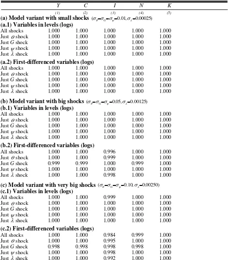
5.2. Comparing the ‘restricted’ versions of the third-order accurate model
Table 2 documents that the ‘restricted’ version (7) of the (pruned) third-order accurate model is observationally equivalent to the ‘unrestricted’ version (5). The correlation between time series
generated by these variants are very close to unity, for GDP, consumption, investment, hours and
the capital stock (both in levels and in first differenced), and that even when shocks are very big.
5.3. Estimating structural parameters and the initial state
I now evaluate the ability of the estimation method to estimate structural model parameters and
latent state variables. For each of the three model variants, I generated 40 simulation runs of
5100 periods (each simulation run was initiated at the unconditional means of the state
10
conducted by maximizing the sum of the likelihood function (10) and a prior log pdf of the initial
state (see below). I estimate the initial states and 10 structural parameters: the risk aversion
coefficient ( ), labor supply elasticity ( ) , as well as the autocorrelations and standard
deviations of the four exogenous variables. As the model has four exogenous shocks, four
observables are needed for estimation. I use first differences of log GDP, consumption,
investment and hours worked as observables.
The model has 5 state variables: the capital stock, and the lagged values of each of the
four exogenous variables. The likelihood depends on the first-, second- and third- order accurate
initial values of these 5 state variables (see (10)). The laws of motion of the four exogenous
variables are log-linear. Hence, their values are identical under (log) approximations of orders
1,2 and 3. To reduce the computational burden, I assume (in the current version of the paper) that
(2) (3) 0 0
k k and (1) (3) (3) (1)
0 0 ( 0 0 );
k k E k k in other terms, the second-order accurate initial state capital
stock is assumed to equal the third-order accurate capital stock; the first-order accurate initial
capital stock is assumed to equal to the third-order accurate initial capital stock, adjusted for the
difference between the mean values of these capital stocks.
The precision of the estimates of the state variables and of the model parameters is higher
if prior information about the mean and variance of the initial state is used. I use a multivariate
normal prior for the initial state vector (lnK0(3),ln0(3),lnG0(3),ln0(3),ln0(3));the prior mean and
covariance are set to the unconditional means implied by the third-order accurate model (7) and
the unconditional covariance implied by the second-order accurate model (4).5
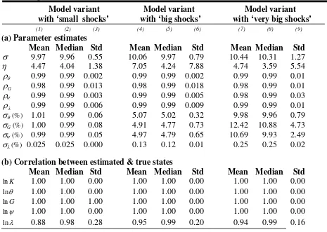
Panel (a) of Table 3 reports the mean, median and standard deviation of the estimated
model parameters across the 40 simulation runs, for the ‘small shocks’ model variant (Columns
(1)-(3)), the ‘big shocks’ variant (Cols. (4)-(6)) and the ‘very big shocks’ model variant (Cols.
(7)-(9)). For each simulation run, I compute the correlation between each estimated state
variables (implied by the estimates of structural model parameters) and the true state variables.
Panel (b) of Table 3 reports the mean, median and standard deviation of the correlation, across
the 40 simulation runs (for each model variant).
Table 3 shows that, for all three model variants, the risk aversion coefficient, the
autocorrelations of the exogenous variables and the standard deviations of exogenous
5
11
innovations are tightly estimated: the mean and median parameter estimates (across runs) are
close to the true parameter values, and the standard deviations of the parameter estimates are
small. The labor supply elasticity is less tightly estimated, in the model variants with ‘big
shocks’ and with ‘very big shocks’, the median estimates (across 40 runs) are close to the true value (4),but the standard deviation of the estimates is sizable.
The estimation method provides remarkably accurate estimates of the 5 state variables.
The estimates of the capital stock, TFP, government purchases and the labor supply shock ( )
are essentially perfectly correlated with the true values of these states, and that irrespective of the
size of the shocks. The shock to the rate of time preference ( ) is somewhat less precisely
estimated; the median correlations between estimates and true values of are 0.98-0.99 (across
12
References
Adjemian, S., H. Bastani, M. Juillard, F. Mihoubi, G. Perendia, J. Pfeifer, M. Ratto, S. Villemot (2014). Dynare: reference manual, Version 4.4.3., Working Paper, CEPREMAP.
An, S. and F. Schorfheide, 2007. Bayesian Analysis of DSGE models. Econometric Reviews 26, 113–172.
Born, B. and J. Pfeifer, 2014. Risk Matters: The Real Effects of Volatility Shocks: Comment. American Economic Review 104, 4231-4239.
Fernández-Villaverde, J. and J. Rubio-Ramírez, 2007. Estimating Macroeconomic Models: a
Likelihood Approach. Review of Economic Studies 74, 1059–1087.
Fernández-Villaverde, J., P. Guerrón-Quintana, J. Rubio-Ramírez and M. Uribe, 2011. Risk Matters: the Real Effects of Volatility Shocks. American Economic Review 101, 2530-2561. Guerrieri, L. and M. Iacoviello (2014). Collateral Constraints and Macroeconomic Asymmetries.
Working Paper, Federal Reserve Board.
Ivashchenko, S. 2014. DSGE Model Estimation on the Basis of Second-Order Approximation. Computational Economics 43, 73-81.
Kim, J., Kim, S., Schaumburg, E. and C. Sims, 2008. Calculating and Using Second-Order Accurate Solutions of Discrete-Time Dynamic Equilibrium Models, Journal of Economic Dynamics and Control 32, 3397-3414.
Kollmann, R., 2004. Solving Non-Linear Rational Expectations Models: Approximations based on Taylor Expansions, Working Paper, University of Paris XII.
Kollmann, R., S. Maliar, B. Malin and P. Pichler 2011. Comparison of Numerical Solutions to a Suite of Multi-Country Models. Journal of Economic Dynamics and Control 35, pp.186-202 Kollmann, R. 2013. Global Banks, Financial Shocks and International Business Cycles:
Evidence from an Estimated Model. Journal of Money, Credit and Banking 45(S2), 159-195. Kollmann, R. 2015a. Tractable Latent State Filtering for Non-Linear DSGE Models Using a
Second-Order Approximation and Pruning, Computational Economics 45, 239-260.
Kollmann, R. 2015b. Tractable Latent State Filtering for Non-Linear DSGE Models Using a Third- Order Approximation and Pruning, work in progress.
Otrok, Christopher. 2001. On Measuring the Welfare Cost of Business Cycles. Journal of Monetary Economics 47, 61-92.
Schmitt-Grohé, S. and M. Uribe, 2004. Solving Dynamic General Equilibrium Models Using a Second-Order Approximation to the Policy Function. Journal of Economic Dynamics and Control 28, 755 – 775.
13
Table 1. RBC model: predicted standard deviations (in%)
Y C I N K
(1) (2) (3) (4) (5)
(a) Model variant with small shocks (
G 0.01,
0.00025)(a.1) Variables in levels (logs)
1st order, all shocks 3.00 1.46 10.35 10.46 7.80 1st order, just shock 2.08 1.37 6.21 9.43 4.58 1st order, just G shock 1.59 0.08 1.46 1.90 1.03 1st order, just shock 1.08 0.70 3.26 0.93 2.32 1st order, just shock 1.68 0.22 7.60 1.55 5.81 2nd order, all shocks 3.09 1.46 10.40 10.45 7.82 3rd order, all shocks 3.04 1.46 10.45 10.44 7.86
(a.2) First-differenced variables (logs)
1st order, all shocks 0.67 0.17 2.62 1.12 0.17
2nd order, all shocks 0.67 0.17 2.62 0.12 0.17 3rd order, all shocks 0.68 0.17 2.63 0.13 0.17
(b) Model variant with big shocks (
G 0.05,
0.00125)(b.1) Variables in levels (logs)
1st order, all shocks 14.99 7.33 51.76 52.31 39.05 2nd order, all shocks 15.89 7.32 53.87 52.29 39.07 3rd order, all shocks 18.71 7.33 60.18 51.62 44.98
(b.2) First-differenced variables (logs)
1st order, all shocks 3.35 0.85 13.09 5.63 0.86 2nd order, all shocks 3.56 0.85 13.45 5.77 0.88 3rd order, all shocks 4.00 0.83 14.63 5.94 0.92
(c) Model variant with very big shocks (
G 0.10,
0.00250)(c.1) Variables in levels (logs)
1st order, all shocks 29.99 14.66 103.52 104.62 78.01 2nd order, all shocks 35.41 14.65 115.43 105.46 86.33 3rd order, all shocks 58.77 14.87 166.39 103.71 123.94
(c.2) First-differenced variables (logs)
1st order, all shocks 6.71 1.70 26.19 11.27 1.72 2nd order, all shocks 7.92 1.71 29.08 12.33 1.86 3rd order, all shocks 11.54 1.63 39.34 14.80 2.21
14
Table 2. RBC model: correlations between variables predicted by ‘full’ and ‘restricted’
versions of third-order accurate model (see (5), (7))
Y C I N K
(1) (2) (3) (4) (5)
(a) Model variant with small shocks ( G 0.01,0.00025)
(a.1) Variables in levels (logs)
All shocks 1.000 1.000 1.000 1.000 1.000
Just shock 1.000 1.000 1.000 1.000 1.000
Just G shock 1.000 1.000 1.000 1.000 1.000
Just shock 1.000 1.000 1.000 1.000 1.000
Just shock 1.000 1.000 1.000 1.000 1.000
(a.2) First-differenced variables (logs)
All shocks 1.000 1.000 1.000 1.000 1.000
Just shock 1.000 1.000 1.000 1.000 1.000
Just G shock 1.000 1.000 1.000 1.000 1.000
Just shock 1.000 1.000 1.000 1.000 1.000
Just shock 1.000 1.000 1.000 1.000 1.000
(b) Model variant with big shocks ( G 0.05,0.00125)
(b.1) Variables in levels (logs)
All shocks 1.000 1.000 1.000 1.000 1.000
Just shock 1.000 1.000 1.000 1.000 1.000
Just G shock 1.000 1.000 1.000 1.000 1.000
Just shock 1.000 1.000 1.000 1.000 1.000
Just shock 1.000 1.000 1.000 1.000 1.000
(b.2) First-differenced variables (logs)
All shocks 1.000 1.000 0.996 1.000 1.000
Just shock 1.000 1.000 0.999 1.000 1.000
Just G shock 0.999 0.999 1.000 0.999 1.000
Just shock 1.000 1.000 1.000 1.000 1.000
Just shock 1.000 1.000 0.998 1.000 1.000
(c) Model variant with very big shocks ( G 0.10,0.00250)
(c.1) Variables in levels (logs)
All shocks 1.000 1.000 0.999 1.000 1.000
Just shock 1.000 1.000 1.000 1.000 1.000
Just G shock 1.000 1.000 1.000 1.000 1.000
Just shock 1.000 1.000 1.000 1.000 1.000
Just shock 1.000 1.000 1.000 1.000 1.000
(c.2) First-differenced variables (logs)
All shocks 1.000 1.000 0.984 0.999 1.000
Just shock 1.000 1.000 0.995 1.000 1.000
Just G shock 0.998 0.998 0.998 0.998 1.000
Just shock 1.000 1.000 0.998 1.000 1.000
Just shock 1.000 1.000 0.992 1.000 1.000
Note: Correlations between variables predicted by the ‘full’ and ‘restricted’ third-order models are reported. ‘All
shocks’: simulations with all 4 shocks. ‘Just shocks’, ‘Just Gshocks’ etc. pertain to simulations in which just
[image:15.612.71.542.101.638.2]15
Table 3. RBC model: estimates of structural parameters and of state variables, 40 simulation runs (100 periods)
Model variant Model variant Model variant with ‘small shocks’ with ‘big shocks’ with ‘very big shocks’
(1) (2) (3) (4) (5) (6) (7) (8) (9)
(a) Parameter estimates
Mean Median Std Mean Median Std Mean Median Std
9.97 9.96 0.55 10.06 9.97 0.79 10.44 10.31 1.27
4.47 4.04 1.38 7.05 4.24 7.88 4.74 3.59 5.54
0.99 0.99 0.002 0.99 0.99 0.002 0.99 0.99 0.01
G
0.98 0.99 0.013 0.98 0.99 0.018 0.98 0.99 0.01
0.99 0.99 0.003 0.99 0.99 0.005 0.98 0.99 0.03
0.99 0.99 0.006 0.99 0.99 0.009 0.99 0.99 0.01
(%) 1.01 0.99 0.06 5.07 5.02 0.32 9.98 9.96 0.79
G
(%) 1.00 0.99 0.08 4.91 4.77 0.73 12.42 10.88 4.73
(%) 0.99 0.99 0.05 4.97 4.79 0.65 10.69 9.93 2.49
(%) 0.025 0.025 0.000 0.13 0.12 0.01 0.25 0.25 0.02
(b) Correlation between estimated & true states
Mean Median Std Mean Median Std Mean Median Std
lnK 1.00 1.00 0.00 1.00 1.00 0.00 1.00 1.00 0.00
ln 1.00 1.00 0.00 1.00 1.00 0.00 1.00 1.00 0.00
lnG 1.00 1.00 1.00 1.00 1.00 0.00 1.00 1.00 0.00
ln 1.00 1.00 0.00 1.00 1.00 0.00 1.00 1.00 0.00
ln 0.88 0.98 0.28 0.95 0.99 0.20 0.94 0.99 0.16
Note: The Table summarizes estimation results across 40 simulation runs of 100 periods each. Panel (a) reports the
mean, median and standard deviation of the estimated model parameters across the 40 runs, for the ‘small shocks’ model variant (Columns (1)-(3)), the ‘big shocks’ variant (Cols. (4)-(6)) and the ‘very big shocks’ variant (Cols. (7)-(9)). For each simulation run, the correlation between the estimated state variables and the true state variables was computed. Panel (b) reports the mean, median and standard deviation of that correlation, across the 40 simulation runs (for each model variant). Mean/median correlations above 0.9995 are reported as 1.00.
The true values of the estimated parameters are: 10, 4, 0.99.
G
In the ‘small shocks’ model variant, the true standard deviations of exogenous innovations are: G 1%, 0.025%.’Big shocks’ model