Abstract— This study proposes an idea of another way of
using utility functions with multi-choice goal programming (MCGP) models. By examining the way the previous study is using utility function with MCGP, some drawbacks of such a way are examined. These drawbacks can mistakenly result in an incomplete representativeness of the original MCGP with utility functions model and thus lead to the inability of the model to appropriately assess and express the real preference structure of a decision maker. This study corrects the way utility functions are used with MCGP. Such a new way is validated by using it to express a decision maker preference structure pertaining to a goal, which underlies his/her real oral statements during decision making.
Index Terms— Multi-choice goal programming, Utility
function, Decision maker, Preference structure, Goal programming
I. INTRODUCTION
ECISION-MAKING (DM) via goal programming (GP) is not news. As a good tool for solving multi-criteria decision making or multi-objective programming, GP has gained its wide popularity [1], since proposed [2].
As a special extension of linear programming, GP was first introduced by Charnes and Cooper, taking into account multiple criteria and achieving multiple objectives. Since then, important extensions and numerous applications have been proposed [3].
The literature is abundant with GP variants (i.e., the GP extension models or specific-purposed formulations for GP). The extension models include, for example, weighted GP (WGP) [4], interactive GP [5], integer GP instead of continuous GP, interval GP (IGP), fuzzy GP (FGP) [6], multi-choice GP (MCGP) [7], multi-segment GP (MSGP) [8], percentage GP (%GP) [9], etc. In addition to these, there are reformulations of either the objective measurement or the goal constraints that can serve as the value-added components of GP to enhance the solving range of GP and to widen the use of GP in different application scenarios. These includes, but not limited to (for space reasons we just list some recent works), dealing arbitrary penalty function for interval programming [10], dealing with the S-shaped penalty function for IGP [11], dealing with procurement risk
using a possibility formulation for fuzzy multi-objective programming [12], weighted max-min model for FGP [13], and so on.
The literature is abundant with applications of GP, too. Over the decades, it has been used to support real-world decision-making processes in many fields such as communication, energy, manufacturing, medical healthcare, vendor selection, pricing, and so on ([14]-[20]).
GP is still popular now and continues to be irrigated by researchers and practitioners [22]. However, the abovementioned GP variants are, in fact, categorized methodologically. When they are categorized through their original ideas, perhaps the article by Tamiz et al. published in 1998 [23], which is an overview of GP modeling techniques that has categorized the considerations, can help.
In the field of GP, as [23] have pointed out, the issues in making the GP variants include Pareto optimality considerations, normalization techniques, the selection of preferential weights and the utility interpretation of GP through utility functions. As can be identified, the last two issues in GP are strongly associated with any DM’s preference structure, so that the works in GP to deal with the DM’s preferences mainly fall in the last two categories.
Studies about modeling the preference structure in GP have also become a subset of GP researches. In 1978, Zimmermann proposed the concept of fuzzy programming (FP) [24], in which the right-hand-side (RHS) of a constraint can be fuzzified with utility functions, and then Narasimhan (1980) applied the “fuzzy subsets” concepts to GP in a fuzzy environment [6]. Martel and Aouni (1990) utilized the Promethee method to build the preference structure of DM for GP and avoided incommensurability problems between criteria that can have various different measurement units [26]. Later, Yang et al. (1991) proposed the fuzzy programming model with non-linear membership functions, using piecewise line segments to approximate the non-linear functions [25]. Mohamed (1997) discussed the relationships (how one can lead to another) between GP and FP [27]. Romero (2004) summarized the general structure of the lexicographic and weighted achievement functions for GP, to deal with the different philosophies of DM preference [4]. Chang (2010) proposed an approximation approach for representing the S-shaped membership functions [28], while Chang (2011) later integrated the concept of utility function into MCGP [29].
To represent the preference structure of DMs, the last model, which is the MCGP with utility function model (hereafter, briefed as the “MCGP+U” model) proposed by Chang [29], involves using multi-choice of RHS values for each goal constraint to represent the multiple goal aspiration levels of a DM. Then the study used utility functions to Ching-Ter Chang and Zheng-Yun Zhuang*
A New Way Using Utility Functions for
Multi-choice Goal Programming Models
D
Manuscript received September 28, 2012; revised January 22, 2013. This work was supported in part by the National Science Council of Taiwan under Grant NARPD3B0052.
C.-T. Chang is the Full Professor and Chair of The Graduate Institute of Business and Management, Chang Gung University.
“glue-up” these RHS values and proposed a model that integrates the ideas of both MCGP and the utility function to solve the decision problem.
Within the MCGP+U model, for a “the-less-the-better” criterion, either the utility function is a purely linear one or a piecewise-linear one (or comes in any other shape else), the utility function always begins with 1 when the achieved goal value is at the minimum bound and it always ends with 0
when the achieved goal value is at the maximum bound. The
situation is vice versa for a “the-less-the-better” criterion. The “maximum and minimum bounds” are defined by the maximal possible aspiration level of a goal and the minimal possible level, among all the multiple choices of aspiration levels.
However, using the utility function in this way can be inappropriate for real-word applications. Take, for example, the slope of the utility function of any specific “the-less-the- better” goal constraint is not necessary to end (to become 0) at the maximum bound of the aspiration levels of a DM. Rather, the location at which the slope of the utility function falls to 0 should depend on a DM’s statement which reveals his/her real preference structure far buried in mind.
Thus, there is a need to change, or revise at least, the way of using utility function with MCGP, so as to reflect the real preference structure of a DM and to correct the possible misleading caused by the previous MCGP+U study.
To have a better understanding about the above core claim mentioned by this study, the way of using the utility function by the original MCGP+U model is examined in Section 2, while the main shortcomings of using a utility function with MCGP in this manner is identified. By observation of some statements of the DMs during decision making, Section 3 proposes a new way of using the utility function with MCGP and examines if such a new way can perfectly express the DM’s preference structure. Section 4 concludes this study.
II. THE WAY UTILITY FUNCTION WAS USED WITH MCGP For simplicity of illustration, the multi-objective numerical decision problem case in Chang’s (2011) study is adopted here, as follow:
(MODM Problem P1) (Goal 1) 8x19x26.5x350 (Goal 2) x10.2x20.5x3 5,
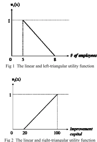
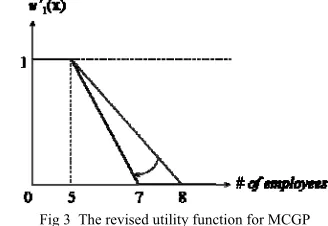
with utility function shown in Figure 1. (Goal 3) 2x13x22.4x3 10,
with utility function shown in Figure 2. (Constraints) 5x17x25.5x340
where x1, x2, x3 are the market share of each product, in
units and should be no less than 2 units; for details please check the original article.
Regardless of what the approach was taken to formulate these utility functions mathematically and to solve the abovementioned decision problem in Chang’s original study [29], there are some facts one can read from these figures.
Firstly, the left- and right- triangles depicted in Figure 1 and 2 represent the two usual types of utility functions (i.e., the-less-the-better and the usual the-more-the-better) that are widely accepted by researchers or practitioners when they are
[image:2.612.341.509.70.316.2]incorporating utility function for solving problems.
Fig 1 The linear and left-triangular utility function
Fig 2 The linear and right-triangular utility function
Secondly, if the real shape of a utility function is not purely linear such as the shapes shown in Figure 1 or 2, they can use the piecewise linear approach to approximate and represent it. In fact, once any utility function is approximated by, or in itself, piecewise line segments, the work left is to find a proper method to model these pieces. For example, Yang et al. [25] proposed a smart approach that uses only 1 binary variable to formulate an S-shaped utility function that is composed of 3 linear pieces. Chang [28] proposed another approach that can deal with an S-shaped utility function which are not purely increasing (concave) or purely decreasing (convex).
Thirdly, as mentioned previously, it may be questionable that such utility functions can fully represent all the facts about a DM’s requirement pertaining to his/her real preference structure, for the reason that it simply bounds the feasible achievement levels of a goal, such as the number of employees goal (i.e., achievement levels are bounded by an interval [5,8]) and the improvement capital (i.e., achievement levels are bounded by [20,100]), with hard constraints.
In real decision cases, the situation for a goal to be achieved outside the sloping range (e.g. the # of employees <5 cases) is very possible and reasonable, if it is more beneficial. That is, allowing the goal achievement to fall in some place outside the defined sloping range is necessary. For example, it can be easily seen that in Figure 1, [0,5] and [8,unlimited) can both be listed as the feasible intervals for Goal 2 to achieve. These two intervals should continuously produce utility levels of 1 and 0, respectively.
multiple possible aspiration levels pertaining to a goal, the range of a utility function to rise up or to slope down (i.e., the “sloping range”) is defined by the maximal and minimal values of these seen levels.
This is not always true, particularly in practice. The “maximum bound” of a utility function defined by Chang in [29] also denotes the maximal seen aspiration level of a goal. However, the maximal seen aspiration level is not equivalent to the point the DM becomes fully unsatisfied (i.e., the end of the sloping range). As can be imagined, the point where the DM becomes fully unsatisfied usually comes earlier than the maximal seen aspiration level.
III. ANEW WAY OF USING UTILITY FUNCTION WITH MCGP By observation of the abovementioned facts, this study suggests another way to use utility function for MCGP. To distinguish this new way from the original way, a thorough dissection is required.
A. The drawbacks of the original way
As can be seen from the fourth observed point, in the original way, when a DM has multiple possible aspiration levels pertaining to a goal, the sloping range of the utility function is usually defined and bounded by the maximum and minimal values of these seen levels.
As discussed previously, under circumstances in practice, the way the MCGP+U model is using utility functions might be ineffective for the sake of the inability to represent a DM’s preference properly. Such a using way might have missed a critical fact that the sloping range should not be defined and bounded by the maximum and minimal values among the multiple, possible aspiration levels of a goal. Instead, it involves the perception of a DM in regard to the durable ranges of that goal.
For example, take the number-of-employees goal in Figure 1 (Goal 2 in the above problem case), if the possible aspiration levels (multiple choices of the RHS) of this goal are 5, 6, 7 and 8, is 8 always the end (downward to exactly 0) of the slope range of the utility function? What if the DM expressed a statement like the following S1?
Statement S1: “A total number of 5, 6, 7, 8 employees are all possible and a total number less than or equal to 5 is strongly acceptable, but for some reasons a total number
greater than 7 is very unacceptable.”
The statement “a total number of 5, 6, 7, 8 employees are all possible” in S1 means that 5, 6, 7, 8 are all possible
choices of the RHS aspiration levels of the goal constraint. But the statement “for some reasons a total number greater than 7 is very unacceptable” means that the end of the sloping range of the utility function to reach 0 is not 8, but 7 instead. With such a consideration, the original way of use of utility function by Chang [29] may distort a DM’s real preference structure and can be infeasible to produce in practice.
Moreover, as can be seen from the third observed point, the sloping range of Goal 2 is closed. That is, only the interval [5, 8] is allowed for Goal 2 to achieve, which is in fact, the sloping range of the utility function exactly. However, inside S1, there is a statement which states that “a total number less than or equal to 5 is strongly acceptable”. This means that a total number of employees under 5 (e.g., 1,
2, 3, or 4, while 0 is quite impossible) also makes the DM perfectly happy. Unfortunately, if a DM had taken the version of utility function in Figure 1, the model could not solve out any answer that leads to 1, 2, 3 and 4 employees just because the utility function is, in itself, bounded by at least 5. This can again distort a DM’s real preference and can be another flaw that deters any practitioner from applying the MCGP+U model.
B. The new way to use utility functions with MCGP
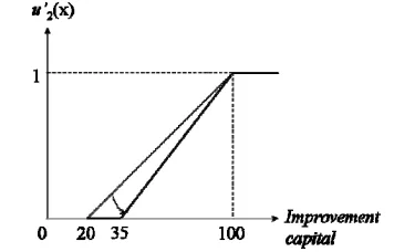
[image:3.612.340.504.210.323.2]Therefore, this study disseminates the idea of making an adjustment to the use of utility function for MCGP. For example, the utility function in Figure 1 can be adjusted as the one shown in Figure 3.
Fig 3 The revised utility function for MCGP
In Figure 3, the single thin solid line, which conforms to Figure 1, is the original version of the utility function u(x)
that described the RHS of Goal 2. As discussed, the feasible range of this goal is bounded by [5,8], which is, exactly, also the sloping range of its utility function.
On the contrary, the bold solid line is the proposed version of the utility function, u1’(x). In compare with u1(x) that contains solely one sloping line segment, u1’(x) has three line segments including one flat segment, one sloping segment and one flat segment that follows, each of which is respectively delimited by x=[0,5), [5,7] and (7,8]. This
relaxes the limitation of the feasible range of Goal 2 that had to be [5,8]. The feasible range of Goal 2 becomes [0,8] instead, to include the possibly forgotten feasible numbers of {0,1,2,3,4} employees, and to include the possible levels of {5,6,7,8} employees, which is the original feasible range of
u1(x).
In addition, as can be seen in Figure 3, within the original feasible range of u1(x), which is [5,8], there are two piecewise
line segments delimited by x=[5,7] and x=(7,8] respectively.
The former part, delimited by x=[5,7], is the interval that
u1’(x) really slopes down. To conform to the statement S1, the sloping range changes from [5,8] (of u1(x)) to [5,7] (of u1’(x)). So the slope should shrink proportionally, no matter what the shape of the slope is (e.g., the linearly-shaped one like this case, or an S-shaped or concave-shaped one for some other cases). The arrow in Figure 3 displays this shrinking process. After shrinking, the slope of the utility function becomes abrupt because the slope range is lessened but the maximal height of the function remains the same (i.e., 1).
The latter tail line segment delimited by x=(7,8] is a flat
segment that produces a satisfaction level of 0. This meets the DM’s claim “but a total number greater than 7 is very unacceptable” in S1. Beware that this formulation, although
aspiration level among the multiple choices of the goal values, so as to faithfully and completely represent the full feasible range in a DM’s mind.
Neglecting this tail part can result in serious consequence. For example, if one excluded this part (i.e., the interval (7,8]) from modeling, the model would have never got an answer that achieves a goal value of 8 for Goal 2, whatever the other constraints are. Consider the case in which a DM is applying MCGP with utility function and there is a must to list 8 as a possible aspiration level of Goal 2 (which implies the achievement of this criterion can be sacrificed when leveraging with other criteria). If the merely the first flat range [0,5) and the slope range [5,7) were taken into account, the model could miss the possible aspiration level of 8, and more critically, would distort the optimal solution because those feasible solutions that achieves Goal 2 with a level of 8 are totally ignored.
In summary, such a new form of u1’(x) can fully describe a DM statement such as S1, and it can be used to denote the real
satisfactory level of a DM more precisely.
At last, let us take a look back to Figure 3 and note a little revision here. In fact, we intentionally let the tail line segment of u1’(x) to penetrate through x=8. This implies that the tail segment can span from 7 to a certain bound or the unlimited (i.e., x=[7, B1] or x=[7, ∞) where B1 is the DM-perceived
upper bound of the x-axis of u1’(x)).
This can be also an important improvement for the original way of use of utility function with MCGP. Such improvement is from the fact that if Goal 2 is not an important goal (e.g., its deviation is not with priority or is assigned a extra low weight in the objective function), a DM can allow it to be “further sacrificed” by extending the tail segment to be ended with 9, 10, 11 and so on, solving the model again and seeing how the optimal solution is changing. For example, a DM’s statement can be S1’ as follows,
rather than S1:
Statement S1’: “For our company, any total number of employees over 8 is able to be exercised and a total number less than or equal to 5 is strongly preferable. But for some internal reasons, a total number greater than 7 is very
unacceptable”.
Shall this be the case, the proposed way of use of utility function in this study, such as u1’(x), can perfectly serve the purpose, while the original way of use, e.g. u1(x), may not.
C. Another example for a “the-more-the-better” criterion
Subsection B demonstrated a new way of using the utility function with MCGP and reshaped the utility function of Goal 2 for its “the-less-the-better”-typed criterion. For a more concrete illustration and a full coverage of the idea of the new using way proposed in this study, an additional case about a goal with a “the-more-the-better”-typed criterion is given.
Consider the capital improvement goal (Goal 3) in P1. The original claim that the DM has made is as follows, which reflects no more than a greedy DM’s prospect:
Statement S2: “A capital improvement between 20M to 100M NT$ is preferred. But for some reasons, an improvement under 35M is quite unacceptable. In fact, any capital improvement level more than 100M is, of course, very
welcomed and I will be fully satisfied with it.”
[image:4.612.331.509.143.257.2]In this case, the sloping range of the utility function in Figure 2 should also shrink, with a front bottom field that produces the altitude (satisfaction level) of 0, followed by an endless Qinghai-Tibet plateau that produces the altitude of 1 consistently. This leads to another new utility function whose shape is quite similar to the topography around Lhasa, as Figure 4 has shown.
Fig 4 The revised utility function for MCGP: the more the better case
IV. CONCLUSION
This study proposes another way of using utility functions when such functions are to incorporate with existing MCGP models.
Some crucial shortcomings when the MCGP+U model is to be applied in practice are examined: the missed ranges of the aspiration levels that the original MCGP+U model might fail to formulate. These missed ranges includes the additional “plain field” range which represents the possible choices of aspiration levels that are acceptable by a DM but can lead to 0 satisfaction of the DM, the “plateau” range which represents the other possible choices of goal levels that makes the DM perfectly happy and the possible extended parts of these ranges. Ignoring these facts during modeling could impair the descriptiveness of the model to represent a DM’s real preference structure.
In consideration of the aforementioned shortcomings, this study proposes the idea of changing the way utility functions are used with a MCGP model. Such a new way to use utility functions with MCGP expresses a DM’s preference structure more precisely. This point is evidential from the fact that the proposed way of using utility function can faithfully formulate the DM statements based on his/her real preference structure pertaining to the goals.
This study also paves ways to future works.
This study changes the way to use utility functions with an MCGP model and studies the topic of “how the using style can be changed”. Although the result of this study is quite interesting, this study does not discuss the topics of “how such a new using style is to be mathematically formulated” as well as of “how the formulation can be incorporated with MCGP”. These become future topics worthy of note.
REFERENCES
[1] B. Aouni and O. Kettani, “Goal programming mode: A glorious history and a promising future,” European Journal of Operational Research, vol. 133, pp. 225-231, 2001.
[2] A. Charnes and W. W. Cooper, “Goal programming and multiple objective optimization,” European Journal of Operational Research, vol. 1, pp. 39-51, 1977.
[3] M. Larbani and B. Aouni, “A new approach for generating efficient solutions within the goal programming model,” Journal of Operational Research Society, vol. 62, pp. 175-182, 2011.
[4] C. Romero, “A general structure of achievement function for a goal programming model,” European Journal of Operational Research, vol. 153, no. 3, pp. 675-686, 2004.
[5] J. S. Dyer, “Interactive goal programming,” Management Science, vol.
19, no.1, pp. 62-70, 1972.
[6] R. Narasimhan, “Goal Programming in a fuzzy environment,” Decision Science, vol. 11, no. 2, pp. 325-336, 1980.
[7] C. T. Chang, “Multi-choice goal programming,” Omega 2007, vol. 35, pp. 389-396, 2007.
[8] C. N. Liao, “Formulating the multi-segment goal programming,”
Computers and Industrial Engineering, vol. 56, pp. 138-141, 2009, [9] C. T. Chang, H. M. Chen and Z. Y. Zhuang, “Revised multi-segment
goal programming: Percentage goal programming”, Computers and Industrial Engineering, vol. 63, pp. 1235-1242, 2012.
[10] H. C. Lu and T. L. Chen, “Efficient model for interval goal programming with arbitrary penalty function,” Optimization Letters
DOI: 10.1007/s11590-011-0422-z, 2011
[11] C. T. Chang and T. C. Lin, “Interval goal programming for S-shaped penalty function,” European Journal of Operational Research, vol. 199, pp. 9-20, 2009.
[12] D. D. Wu, Y. Zhang, D. Wu and D. L. Olson, “Fuzzy multi-objective programming for supplier selection and risk modeling: A possibility approach,” European Journal of Operational Research, vol. 200, pp. 774-787, 2010.
[13] C. C. Lin, “A weighted max-min model for fuzzy goal programming,”
Fuzzy Sets and Systems, vol. 142, pp. 407-420, 2010.
[14] J. T. Blake and M. W. Carter, “A goal programming approach to strategic resource allocation in acute care hospitals,” European Journal of Operational Research, vol. 140, no. 3, pp. 541-561, 2002. [15] E. A. Demirtas and O. Ustun, “Analytic network process and
multi-period goal programming integration in purchasing decisions,”
Computers and Industrial Engineering, vol. 56, no. 2, pp. 677-690, 2009.
[16] H. W. Lin, S. V. Nagalingam and G. C. I. Lin, “An interactive meta-goal-programming-based decision analysis methodology to support collaborative manufacturing,” Robotics and Computer- Integrated Manufacturing, vol. 25, no. 1, pp. 135-154, 2009.
[17] J. E. Samouilidis and I.A. Pappas, “A goal programming approach to energy forecasting,” European Journal of Operational Research, vol. 5, no. 5, pp. 321-331, 1980.
[18] P. Korhonen and M. Soismaa, “A multiple criteria model for pricing alcoholic beverages,” European Journal of Operational Research, vol. 37, no. 2, pp. 165-175, 1988.
[19] J. A. Gómez-Limón and L. Riesgo, “Irrigation water pricing: differential impacts on irrigated farms,” Agricultural Economics, vol.
31, no. 1, pp. 47-66, 2004.
[20] K. Senthilkumar, M. T. M. H. Lubbers, N. De Ridder, P. S. Bindraban, T. M. Thiyagarajan and K.E. Giller, “Policies to support economic and environmental goals at farm and regional scales: Outcomes for rice farmers in Southern India depend on their resource endowment,”
Agricultural Systems, vol. 104, no. 1, pp. 82-93, 2011.
[21] M. Tamiz, D. F. Jones and C. Romero, “Goal programming for decision making: an overview of the current state-of-the-art,” European Journal of Operational Research, vol. 111, no. 3, pp. 569-581, 1998.
[22] B. Aouni and D. La Torre, “A generalized stochastic goal programming model,” Applied Mathematics and Computation, vol. 215, no. 12, pp. 4347-4357, 2010.
[23] M. Tamiz, D. Jones and C. Romero, “Goal programming for decision making: An overview of the current state-of-the-art,” European Journal of Operational Research, vol. 111, pp. 569-581, 1998. [24] H. J. Zimmermann, “Fuzzy programming and linear programming with
several objective functions,” Fuzzy Sets and Systems, vol. 1, pp. 45-55,
1978.
[25] T Yang, J. P. Ignizio and H. J. Kim, “Fuzzy programming with nonlinear membership function: Piecewise linear approximation,”
Fuzzy Sets and Systems, vol 41, pp. 39-53, 1991.
[26] J. M Martel and B. Aouni, “Incorporating the decision-maker’s preference in the goal-programming model,” The Journal of the Operational Research Society, vol. 41, no. 12, pp. 1121-1132, 1990.
[27] R. H. Mohamed, “The relationship between goal programming and fuzzy programming,” Fuzzy sets and systems vol. 89, pp. 215-222, 1997.
[28] C. T. Chang, “An approximation approach for representing S-shaped membership functions,” IEEE Transaction of Fuzzy Systems, vol. 18, no. 2, pp. 412-424, 2010.
[29] C. T. Chang, “Multi-choice goal programming with utility function,”