Abstract—Multi-class classification models commonly hide more complex patterns from discrimination. Multi-class classification problems challenge many traditional classifiers to select a set of characterizing features. In fact, the authentication of features’ discrimination capability should be prior to proceeding feature selection. The enhancement of features’ discrimination power using fuzzy clustering analyses is proposed in this paper. In addition, a set of low-dependent features capable of collecting the enough data variability is selected for the completeness of classification tasks. Experimental results show that the classification models adopting our schemes can gain performance improvement.
Index Terms—Feature selection, discrimination power,
cluster analysis, multi-class classification
I. INTRODUCTION
he goal of classifier is to accurately predict the target class for each instance in the dataset. Generally, classifications are discrete and do not imply order. The simplest type of classification problem is binary and the target classes are alternative. Multiclass targets have more than two values and impose more intricate tasks on multiclass classification problems. In model building process, an inductive learning algorithm takes the responsibility of finding relationships between the values of the predictors and the values of the target. Different models exercise distinct techniques for the exploration of inherent but implicit relationships. The common goal is to discover the crucial classification factors or the serviceable decision rules.
It is difficult for any single variable to distinguish multiple classes to their fullest. In general, one class is satisfied while other classes suffer as a result. Classification problems with multiple classes introduce perplexing interaction among features and such situation necessitates more efforts in data processing. Scaling up for high dimensional data and high speed streams have pushed the complexities of classification problems to the even higher boundary. Tremendous amount of ultra high dimensional data become ubiquitous and they impose heavy analytical and computational overheads on current data mining tasks.
Features are typically expressed by categorical, nominal, or numerical values. The diversity of feature values in categorical and nominal types is simply limited. However, the diversity of numerical data is much greater due to their
This research was supported by Nation Science Council of ROC under Grant 101-2221-E-025 -012. Hung-Yi Lin is now an associate professor with the Department of Distribution Management, National Taichung University of Science and Technology, Taiwan R.O.C., (e-mail: [email protected]).
continuity or multiplicity, especially when floating-point values are involved. Numerical features usually require preprocessing for data simplicity. The purpose of simplicity has two effects. Avoidance of mess information on computational process is the first. The second is to prevent outlier or noisy data from being involved in the analytical process.
Feature evaluation makes preparation for feature selection; nevertheless, precise feature evaluation greatly relies on the preprocessing quality of feature values. Adequate feature preprocessing can exhibit features’ discrimination powers and in turn lead to precise feature evaluation. A well preprocessing scheme can not only achieve data simplicity but also retain data characteristics including distribution, variation, and proximity. The enhancement of discrimination power for every feature is the first goal of this paper. However, combinations of individually good features do not necessarily lead to good classification performance. The second goal is to generate a compact subset of features which maximizes the discriminative effect for the target decision concept.
This paper is organized as follows: next section the fuzzy c-means algorithm and PBMF-index are sketched. A new feature evaluation criterion using cluster analysis is presented in Section 3. A self-explanatory example is also provided in this section. The novel feature selection algorithm is explained in Section 4. The experimental and analytical results are presented in Section 5. Finally, concluding remarks are given in the last section.
II. FUZZY C-MEANS AND PBMF-INDEX
Fuzzy c-means (FCM) algorithm proposed by [1] adopts fuzzy logic which is similar to human reasoning. It allows one piece of data to belong to two or more clusters. Consider the dataset T={xi| 1≤i≤N }, where each sample contains p-dimensional vector p
i
R
x
∈
. The algorithm aims to find a fuzzy partition of the domain into a set of K clusters {C1… CK}, where each cluster Cj is represented by its center’s coordinates’ vector pj R
v ∈ . Each sample in the training set
can be assigned to more than one cluster, according to a value ij
u
, that defines the membership of the sample xi to the cluster Cj.FCM algorithm computes the centers’ coordinates by minimizing the objective function Jm defined as:
∑∑
= =
− × =
N
i K
j
j i m ij
m u x v
J
1 1
2 (1)
, where m>1 is referred as the fuzziness parameter and used to adjust the effect of membership values. The norm
j
i
v
x
−
is a distance measure from the sample xi to the cluster’s center vj. The membership of all samples to all clusters defines a partition matrix as:Effective Feature Selection for Multi-class
Classification Models
Hung-Yi Lin,
Member, IAENG
= NK N K u u u u U L M O M L 1 1 11 (2)
The partition matrix is computed by the algorithm and the summation of
ij
u in each row is equal to 1. The FCM algorithm computes interactively the cluster centers’ coordinates from a previous estimate of the partition matrix as:
∑
∑
= = = N i m ij N i i m ijj u x u
v 1 1 (3) The membership ab
u in the partition matrix is updated as: 1 ) 1 ( 1 1 ] ) ( [ − − =
∑
− − = m Kj a j
b a ab v x v x
u , 1≤a≤Nand 1≤b≤K (4)
The FCM algorithm is described as follows:
1. Set m>1, K≥2 and initialize the cluster centers’ coordinates randomly, initialize the partition matrix as (4).
2. For all clusters, update cluster centers’ coordinates as (3). 3. For all samples and all clusters, update the partition
matrix as (4).
4. Stop when the norm of the overall difference in the partition matrix between the current and the previous iteration is smaller than a given threshold; otherwise go to step 2.
The computation of cluster centers’ coordinates and the partition matrix depend on the specification of the number of clusters K. Two typical clustering questions are frequently addressed: (i) how many clusters are actually present in the data and (ii) how good is the clustering itself. The problem in finding an optimal number of clusters is called the cluster validity problem [2]. A number of clustering methods [9, 10] and validation indices [14, 15] have been proposed and successfully employed to solve this problem. The PBMF-index [10] is employed to verify the quality of FCM cluster analysis in this paper.
The PBMF-index is defined as a product of three factors. The product with maximization ensures the partition has a small number of compact clusters with large separation between at least two clusters. Mathematically, the PBMF-index for K clusters is defined as follows:
2 ) 1 ( ) ( K m PBMF D J E K K
V = ⋅ ⋅ (5)
The factor E is the sum of the distances of each sample to the geometric center v0. This factor does not depend on the number of clusters and is computed as:
∑
= − = N i i v x E 1 0 (6)The factor Jm is the sum of within cluster distances of K clusters, weighted by the corresponding membership value and the same as that in the FCM algorithm. DK represents the maximum separation of each pair of clusters:
j i K j i
K v v
D = −
≤ ≤, 1max
(7) The optimizing of PBMF-index relies on the fewer cluster number, the lower measure of Jm (i.e., the best clustering fuzzy partition), and the higher estimation of DK. The calculation procedure is explorative and described as follows:
1. Compute the PBMF factor E as (6); 2. K1←2;
3. K2←K1+1;
4. Run the FCM algorithm; 5. Compute the PBMF factors Jm,
1 K D , and
2 K
D as (1) and (7);
6. Compute the VPBMF(K1)and VPBMF(K2) as (5);
7. Stop when VPBMF(K1) is greater than VPBMF(K2)and return VPBMF(K1); otherwise K1←K1+1and go to step 3.
Although such explorative search could fall into the local optimization where only small cluster numbers are investigated, features classified into an adequate small number of categorization is sufficient and highly expected for the reason that over-fitting problems can be kept off.
III. FEATURE EVALUATION
Classification problems relying on a large set of continuous features tend to be overly categorized. To get rid of this situation, continuous features usually necessitate preprocessing. In machine learning, discretization refers to the process of converting or partitioning continuous features to discretized or nominal features. This can be useful when creating probability mass functions. Typically, data is discretized into partitions of P equal lengths/width (equal intervals) or P% of the total data (equal frequencies). Some machine learning algorithms [12, 16] are known to produce better models by discretizing continuous features. As far as classification problems are concerned, the enhancement of discrimination power is prior to all other factors.
As proposed in [8], an enhanced entropy-based criterion called aggregation gain (AG) can precisely evaluate features by taking data variation into consideration, besides the information about data distribution. The AG criterion is particularly powerful when multiple classes are handled. In this paper, the continuous features preprocessed by FCM and validated by PBMF-index are evalauted by AG criterion. In order to present a convincing argument, a small dataset as an illustrative example is used to demonstrate how features’ discrimination powers are improved by fuzzy cluster analysis. The 25 instances are randomly extracted from the glass identification dataset [17] which was motivated by criminological investigation. As shown in Table I, the glass fragments left at the scene are analyzed by physical and chemical test and then some measured numeric data are preserved.
TABLEI
RAW DATA EXTRACTED FROM GLASS IDENTIFICATION DATASET
No. Refractive
index (a1)
Magne-
sium(a2)
Alumi-
num(a3)
Silicon (a4)
Potas-
sium(a5)
Calcium (a6)
Barium (a7)
Type (O)
10 1.53393 12.3 0 1 70.16 0.12 16.19 2 11 1.51905 14 2.39 1.56 72.37 0 9.57 5 12 1.51514 14.01 2.68 3.5 69.89 1.68 5.87 4 13 1.52121 14.03 3.76 0.58 71.79 0.11 9.65 3 14 1.51918 14.04 3.58 1.37 72.08 0.56 8.3 1 15 1.51852 14.09 2.19 1.66 72.67 0 9.32 5 16 1.51545 14.14 0 2.68 73.39 0.08 9.07 6 17 1.51623 14.14 0 2.88 72.61 0.08 9.18 6 18 1.51916 14.15 0 2.09 72.74 0 10.88 5 19 1.51768 12.65 3.56 1.3 73.08 0.61 8.69 1 20 1.52213 14.21 3.82 0.47 71.77 0.11 9.57 1 21 1.52777 12.64 0 0.67 72.02 0.06 14.4 2 22 1.52369 13.44 0 1.58 72.22 0.32 12.24 4 23 1.51969 14.56 0 0.56 73.48 0 11.22 5 24 1.52365 15.79 1.83 1.31 70.43 0.31 8.61 6 25 1.51838 14.32 3.26 2.22 71.25 1.46 5.79 6
Common processing of discretization simply partitions the underlying data domain of continuous feature into some equal divisions with a fixed interval length. As shown in Table II(a), all features are discretized into five grades and five grades are adopted because there are only six classes in the target classification variable. Taking feature a1 as an illustration, the mapped feature is denoted as
a
1'
and regulated as follows: for] 5 , 4 , 3 , 2 , 1 [ ∈
s , if 1.511+0.004s<a1≤1.515+0.004s , then s
a1'= .
On the other hand, Table II(b) lists the raw features processed by FCM and validated by PBM-index. Distinct cluster numbers varying from 3 to 6 are generated for different features. The underlying data domain of every feature is divided into unequal parts with uneven interval length. Again, taking feature a1 as an illustration, cluster analysis categorizes data as follows:
∈
1
a
[1.515, 1.520], a1''=1∈
1
a
(1.520, 1.525], a1''=2∈
1a
(1.525, 1.535],a
1''
=
3
TABLEII
(A)SIMPLE-DISCRETIZATION (B)CLUSTER-DISCRETIZATION
Figure 1 shows the difference between simple and clustered discretization. The graduations are depicted on the horizontal axes. The vertical axes are used to prevent the data points from mixing. Obviously, simple discretization probably
separates the similar data and categorizes the dissimilar data into the same cluster. FCM can take data proximity, sociality, and distribution into account.
(a) Simple-discretization
[image:3.595.56.283.50.204.2] [image:3.595.306.546.89.265.2](b) Cluster-discretization
Fig. 1. Difference between simple- and cluster-discretizations.
To verify the effect of cluster analysis upon the discrimination power, information gain (IG) and aggregation gain (AG) are applied for these seven features of this example. Regarding the IG part of Table III, the rank orders of simple- and cluster-discretizations are so different that features a4" and a3" own the highest rank and gain the most apparent IG improvement of all. The average IG for all ai" is better than that for all ai'. As to the AG part, the most characterizing features get the highest measures and are consistently classified by two discretization methods. In short, cluster-discretization cooperated with AG criterion explicitly approve the third and fourth features as the characterizing features.
TABLEIII
MEASURES OF IG AND AG FOR SEVEN FEATURES
Rank IG AG
1 a1' 0.90 a4" 1.43 a3' 3.92 a3" 4.99
2 a7' 0.85 a3" 1.34 a4' 3.16 a4" 4.58 3 a3' 0.80 a1" 0.80 a6' 2.62 a5" 2.62 4 a2' 0.72 a7" 0.69 a2' 2.53 a1" 2.51 5 a4' 0.68 a2" 0.58 a1' 2.39 a6" 2.04 6 a5' 0.59 a5" 0.56 a7' 2.06 a2" 1.93 7 a6' 0.49 a6" 0.52 a5' 1.84 a7" 1.68
Avg. 0.72 0.85 2.65 2.91
IV. SELECTION ALGORITHM
We investigate a two-stage selection process. Relevant and irrelevant features are distinguished using the AG-based criterion at the first stage. Features classified as irrelevant are removed from the classification tasks. Relevant features become the candidates for the selection of characterizing features. A categorization suggestion is based on the average of all AG’s. At the second stage, a learning model using multivariate analysis is schemed out to boost the joint discrimination power of earlier selected features. The effect of the features subsequently selected is based on their complementary discriminative effect but not their individual discrimination powers.
For the completeness of learning model, we present below the algorithm of feature selection in detail. The notations used in the algorithm are first listed as follows:
A: The set contains all original features and the set size No. a1' a2' a3' a4' a5' a6' a7' No. a1'' a2'' a3'' a4'' a5'' a6'' a7''
1 5 1 1 3 1 2 4 1 3 1 1 6 1 2 3 2 4 1 1 1 4 1 5 2 3 1 1 2 4 1 3 3 2 1 2 2 4 2 3 3 2 1 2 5 5 2 2 4 4 4 4 1 1 1 3 4 3 3 5 2 1 1 2 5 3 3 4 1 2 1 3 5 2 3 6 1 3 1 2 6 2 1 2 2 3 1 3 6 2 1 2 5 4 2 2 7 1 2 1 2 5 5 2 7 1 2 1 3 5 4 1 8 1 2 4 2 3 2 2 8 1 2 6 4 4 2 1 9 1 2 4 2 4 2 2 9 1 2 5 3 5 2 1 10 5 2 1 1 1 1 5 10 3 2 1 3 1 1 3 11 2 4 3 2 3 1 2 11 1 3 3 5 3 1 1 12 1 4 3 5 1 4 1 12 1 3 4 7 1 3 1 13 2 4 4 1 2 1 2 13 2 3 6 1 3 1 1 14 2 4 4 2 3 2 2 14 1 3 6 4 3 2 1 15 1 4 2 2 3 1 2 15 1 3 3 5 4 1 1 16 1 4 1 4 4 1 2 16 1 3 1 7 5 1 1 17 1 4 1 4 3 1 2 17 1 3 1 7 4 1 1 18 2 4 1 3 3 1 3 18 1 3 1 6 4 1 2 19 1 2 4 2 4 2 2 19 1 2 6 4 4 2 1 20 2 4 5 1 2 1 2 20 2 3 6 1 3 1 1 21 4 2 1 1 3 1 5 21 3 2 1 2 3 1 3 22 3 3 1 2 3 1 4 22 2 3 1 5 3 2 2 23 2 4 1 1 4 1 3 23 1 3 1 1 5 1 2 24 3 5 2 2 1 1 2 24 2 4 2 4 1 2 1 25 1 4 4 3 2 3 1 25 1 3 5 6 2 3 1
a1'=1 a1'=2 a1'=3 a1'=4 a1'=5
exceeds 2.
C: The set contains candidate features.
B: The initial feature basis for variability analysis.
λ
1(S): Apply principle component analysis (PCA) to Sand extract the first eigenvalue from the corresponding correlation matrix.
1. Sort all features in A according to their AGs in a decreasing order. If two or more features have the same evaluation, the feature with higher priority is ranked first. The feature with the highest AG is denoted as a1 and so forth.
2. n← |A|. /* Designate a maximum selection quantity
of features */
3. C← {a1, a2, a3, …, an} /* The first n features in A are taken as candidates */
4. According to practical demand or users’ requirement, pick a small number of characterizing features from C and collect them into B.
5. While B <nand C−B≠φdo
6. For every feature
a
iin C-B, calculate λ1(BU{ai}). 7. Select the next characterizing featureα
by})) { ( ( max
arg 1 i
B C a
a B i
U
λ
− ∈
8. B←BU{α}
9. End For 10. End While 11. Return B.
Step 2 designates a maximum selection number and this assignment ensure a sufficient amount when |A|<10. This assignment is only a suggestion derived from statistical sampling and users can adjust it according to their practical requirements. A small number of features is selected and collected into set B as described at step 4. The selection of the next characterizing feature appeals to multivariate analysis as outlined from step 5 to 9. Step 5 monitors the whether the maximum selection number is reached and whether any feature remains for next selections. For any feature possibly serviceable to the classification task, step 6 calculates the first eigenvalues for the feature combination and step 7 selects the feature with the best variability contribution to set B.
Again, taking the glass dataset as an illustration, our algorithm selects a1", a3", and a4" as the final charactering features. We measure the classification performance achieved by {a1", a3", a4"} in terms of accuracy rate when compared with that achieved by {a1', a3', a7' }. As shown in Table IV, for
classifiers C4.5, NaïveBayes, and SVM, the accuracy improvements of 23%, 78%, and 60% are obtained in this example.
TABLEIV ACCURACY COMPARISON (%)
{a1', a3', a7' } {a1", a3", a4"}
C4.5 52.2 64.8
Naïve Bayes 36.3 63.5
SVM 40.2 63.2
V. EXPERIMENTAL RESULTS AND ANALYSES A. Dataset Acquisition
Five datasets used in this paper are glass, svmguide4, vehicle, segment, and satimage which are downloaded from [17], StatLib [3, 18], and Statlog [19]. Table V depicts the abstract of five datasets. The number of features varies from 9 to 36 and the number of target classes varies from 4 to 7. For simplicity, five datasets are respectively denoted as DS1, DS2, DS3, DS4, and DS5. The data type of all features in the five datasets is either continuous or nominal. Continuous features in all datasets were preprocessed by FCM and the resulting cluster numbers were validated by PBMF-index. Nominal features with ordinal values were analyzed in a similar way. We note that a great number of nominal values could be simplified to a reduced number of categorizations. However, a small number of nominal values could retain their original values after applying cluster analysis. All decision models were implemented in C and Matlab programming languages executed on a workstation with an AMD Athlon dual core 2.59 GHz processor. To verify our design, three classification methods including C4.5, NaiveBayes(NB), and SVM are selected from the 10 most influential algorithms [13] and used in the comparison experiments.
TABLEV ABSTRACT OF FIVE DATASETS
Datasets (DS1) glass svmguide4 (DS2) vehicle (DS3) segment (DS4) satimage (DS5)
# of instances 214 612 946 2310 6455
# of features 9 10 18 19 36
# of classes 6 4 4 7 6
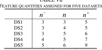
According to our selection algorithm, the numbers of candidate features for the five datasets were respectively initialized as 9, 10, 18, 19, and 36; i.e., n=3, 4, 5, 5, and 6. The dependencies among the features qualified by IG and AG were first investigated. That is, the first n features with the best IG and AG values are respectively extracted and the absolute correlation coefficients for every pair of them are calculated and averaged. As shown in Table VI, AG can classify the features with lower correlation degree than IG no matter simple- or cluster- discretization is applied.
TABLEVI FEATURE DEPENDENCY
IG AG
Datasets simple clustered simple clustered DS1 0.324 0.379 0.449 0.489 DS2 0.578 0.619 0.489 0.434 DS3 0.827 0.845 0.820 0.845 DS4 0.540 0.978 0.192 0.506 DS5 0.807 0.803 0.821 0.632 Average 0.615 0.725 0.554 0.581
Three quantities are respectively formulated as
|A|2
n−= ,
| |
An= , and n+ =
|2A|
for theleast feature number of all, the values of
n
−andn
are the same.TABLEVII
FEATURE QUANTITIES ASSIGNED FOR FIVE DATASETS
−
n
n
n
+DS1 3 3 5
DS2 3 4 5
DS3 3 5 6
DS4 4 5 7
DS5 5 6 9
B. Accuracy Studies
Let us look at the performance of classifiers built by the features selected in this paper. For convenience of explanation, let SD and CD respectively stand for the features selected via the preprocessing of simple-discretization and clustered-discretization. In addition, CDH indicates the features selected via the processing of cluster-discretization cooperated with the our selection algorithm. For SD and CD, the features with the better IGs and AGs are collected for the classification problems. CDH requires more computational costs in the collection of relevant features than SD and CD. Three strategies (SD, CD, and CDH) were applied to the five datasets (DS1~DS5) when three selection quantities ( −
n
,n
, and +n
) were assigned. All experimental results in this study were assessed using 10-fold cross-validation. Figures 2~4 respectively depict the classification accuracies using C4.5, NB, and SVM classifiers. For all cases, cluster analyses successfully improve the discrimination powers of selected features and in turn lead to the better accuracy with the improvement of 24% in average. We note that DS2, DS4, and DS5 have more significant improvement than others. DS2 and DS4 respectively improve 64% and 34% accuracies. Furthermore, CDH acquires a slight improvement of 2% in average when compared with CD. DS1 acquires the highest improvement of 6% of all. Since the amounts of features selected in these five datasets are not so great (<10) that the effect of our selection method is insignificant. However, C4.5 and SVM using CDH still benefit by the effect of multivariate analysis. The performance of DS3 display thatn
[image:5.595.305.541.59.162.2]outperforms
n
− andn
+ in cases of CD and CDH. The insufficient data quantity could be the cause of inconsistency happened to DS1.Fig. 2. Accuracies of C4.5.
Fig. 3. Accuracies of NB.
Fig. 4. Accuracies of SVM.
C. Performance of Different Selection Schemes
To prove the usefulness of our CDH method, five well-known feature selection schemes including Information Gain (IG), Chi-Squared (
χ
2), Correlation-based Feature Selection (CFS) [5], Relief-F [7], and Simba [6] are employed in the final comparison experiment. Rather than merely scoring individual features, CDH, CFS, ReliefF, and Simba methods analyze (or evaluate) the worth of subsets of features. The data complexity involved in the execution of CDH is) (NM
O , where N is the initial number of features and M is the instance number in the original dataset. The CFS method requires O((N2−N) 2)×M) operations [4] for computing the pairwise feature correlation matrix. Hence, the computational cost of CDH is more economic than that of CFS. Relief-F's asymptotical complexity [11] is
O
(
TNM
)
, where T is a user-defined parameter for the greater robustness of the algorithm concerning noise and controls the locality of the estimates. Relief-F has no mechanism for eliminating redundant features. Simba may also choose correlated features. The computational complexity of Simba is equivalent to Relief-F and their computational costs are higher than CDH.To have a fair comparison baseline, the number of candidate feature used in the training processes of C4.5, NB, and SVM are again initialized as n=
|A|
, i.e., 3, 4, 5, 5,and 6, respectively. The 10-fold cross-validation classification accuracies (%) followed with ROCs for five classifiers are respectively listed from Tables VIII to X. The CDH method explicitly outperforms the IG and χ2 methods in the aspects of classification accuracy and discrimination power. Approximately, 30% accuracy improvement and 10% discrimination improvement are obtained. When comparing with CFS, Relief-F, and Simba, the discrimination power derived from CDH outperforms that derived from CFS, Relief-F, and Simba. The average gain is about 10%. As to classification accuracy, although CDH does not significantly outperform CFS, Relief-F, and Simba, it is very competitive to them.
TABLEVIII
PERFORMANCE OF FOUR FEATURE SELECTION SCHEMES FOR C4.5
IG χ2 CFS Relief-F Simba CDH
DS1 48.2[0.71] 51.8[0.72] 64.7[0.87] 71.8[0.76] 73.2[0.78] 70.6[0.84]
DS2 43.6[0.69] 54.7[0.79] 70.2[0.78] 73.4[0.79] 73.8[0.81] 72.5[0.89]
DS3 40.5[0.62] 42.2[0.69] 58.3[0.83] 65.2[0.72] 65.9[0.74] 64.3[0.83]
DS4 71.4[0.92] 74.6[0.92] 93.2[0.92] 94.2[0.88] 94.8[0.89] 94.7[0.99]
DS5 80.5[0.94] 82.3[0.93] 86.2[0.85] 95.7[0.89] 95.2[0.89] 95.8[0.99]
[image:5.595.86.252.96.178.2] [image:5.595.48.284.589.775.2]TABLEIX
PERFORMANCE OF FOUR FEATURE SELECTION SCHEMES FOR NB
IG χ2 CFS Relief-F Simba CDH
DS1 39.8[0.62] 38.6[0.65] 61.2[0.79] 65.7[0.72] 65.9[0.76] 63.6[0.83]
DS2 42.2[0.69] 53.4[0.81] 68.1[0.80] 65.4[0.72] 68.5[0.77] 66.5[0.88]
DS3 38.7[0.66] 42.5[0.73] 56.8[0.81] 58.7[0.76] 60.6[0.79] 55.1[0.79]
DS4 69.0[0.91] 74.8[0.90] 92.4[0.91] 88.6[0.87] 90.6[0.87] 88.2[0.99]
DS5 74.3[0.94] 72.6[0.87] 77.9[0.85] 90.5[0.89] 92.6[0.89] 92.9[0.99]
Avg. 52.8[0.77] 56.4[0.79] 71.3[0.83] 73.8[0.79] 75.6[0.82] 73.3[0.90]
TABLEX
PERFORMANCE OF FOUR FEATURE SELECTION SCHEMES FOR SVM
IG χ2 CFS Relief-F Simba CDH
DS1 52.6[0.81] 51.7[0.81] 68.4[0.88] 72.5[0.80] 72.2[0.77] 69.2[0.82]
DS2 43.3[0.67] 54.9[0.83] 71.0[0.74] 72.6[0.79] 72.8[0.85] 70.9[0.90]
DS3 46.2[0.71] 45.8[0.73] 63.7[0.82] 65.4[0.74] 62.7[0.76] 61.6[0.78]
DS4 70.0[0.90] 68.8[0.87] 93.3[0.94] 90.8[0.86] 91.6[0.88] 93.5[0.98]
DS5 80.2[0.93] 76.3[0.85] 87.6[0.86] 97.8[0.85] 96.3[0.89] 97.3[0.99]
Avg. 58.5[0.81] 59.5[0.82] 76.8[0.85] 79.8[0.81] 79.1[0.83] 78.5[0.90]
VI. CONCLUSIONS
The main contributions of this paper are threefold. First, the enhancement of discrimination power facilitates the authentication of characterizing features. Cluster analyses using fuzzy c-means is proposed for this goal. Second, a novel feature selection algorithm capable of exploring the suitable subset of features with the necessary and sufficient information for classification is proposed. Variability analyses using PCA was taken to fulfill this goal. Third, our algorithm has the accessory effect that the selected features are lowly correlated with each others. Such effect prevents redundant classification handles from being repeatedly executed.
REFERENCES
[1] J. C. Bezdek, “Pattern Recognition with Fuzzy Objective Function Algorithms,”Kluwer Academic Publishers Norwell, MA, USA, 1981. [2] J. C. Bezdek,. “Cluster validity with fuzzy sets,” Journal of Cybernetics
3(3), pp. 58-73, 1973.
[3] C. C. Chang, and C. J. Lin, Software available: a library for support vector machines (LIBSVM). http://www.csie.ntu.edu.tw/~cjlin/libsvm, 2001.
[4] T. Fawcett, “An introduction to ROC analysis,” Pattern Recognition Letters 27: pp. 861-874, 2006.
[5] Y. Feng,Z. Wu, X.Zhou, Z. Zhou, and W. Fan,“Knowledge discovery in traditional Chinese medicine: State of the art and perspectives,” Artificial Intelligence in Medicine 38(3), pp. 219-236, 2006. [6] R. Gilad-Bachrach, A. Navot, and N. Tishby, “Margin based feature
selection-theory and algorithms,” In Proceedings of the 21th Int. Conf. on Machine learning, 2004.
[7] I. Kononenko, Estimating attributes: “Analysis and extensions of Relief,” In Proceedings of the European Conference on Machine Learning, pp. 171-182, 1994.
[8] H. Y. Lin, “Efficient classifiers for multi-class classification problems,” Decision Support Systems 53(3), pp. 473-481, 2012. [9] R. Nock, and F. Nielsen, “On weighting clustering,” IEEE
Transactions on Pattern Analysis and Machine Intelligence 28(8), pp. 1223-1235, 2006.
[10] M. K. Pakhira, S. Bandyopadhyay, and U. Maulik, “A study of some fuzzy cluster validity indices, genetic clustering and application to pixel classification,” Fuzzy Sets Systems 155, pp. 191-214, 2005. [11] M. Robnik-Šikonja, and I. Kononenko, “Theoretical and empirical
analysis of ReliefF and RReliefF,” Machine Learning 53(1-2), pp. 23-69, 2003.
[12] K. Shehzad, EDISC: “A class-tailored discretization technique for rule-based classification,” IEEE Transactions on Knowledge and Data Engineering 24(8), pp. 1435-1447, 2012.
[13] X. Wu, V. Kumar, J. R. Quinlan, J. Y. Ghosh, Q., M. H., G. McLachlan, et al. “Top 10 algorithms in data mining,” Knowledge and Information Systems 14(1), pp. 1-37, 2008.
[14] K. L. Wu, and M. S. Yang, “A cluster validity index for fuzzy clustering,” Pattern Recognition Letters 26(9), pp. 1275-1291, 2005. [15] Y. Zhang, W. Wang, X. Zhang, and Y. Li, “A cluster validity index for
fuzzy clustering,” Information Sciences 178(4), pp. 1205-1218, 2008. [16] Q. Zhu, L. Lin, M. L. Shyu, and S. C. Chen, “Effective supervised discretization for classification based on correlation maximization,” IEEE International Conference on Information Reuse and Integration: pp. 390-395, 2011.
[17] UCI Learning Repository,