Normal zone propagation in a YBCO superconductor at 4 2 K and above

(1)

MASTER THESIS

NORMAL ZONE

PROPAGATION IN A YBCO

SUPERCONDUCTOR AT 4.2 K

AND ABOVE

A.R. Hesselink

FACULTY OF SCIENCE AND TECHNOLOGY ENERGY, MATERIALS AND SYSTEMS GROUP EXAMINTATION COMMITTEE

Dr. M.M.J. Dhallé

(2)

Abstract

(3)

Chapter 1 Introduction

This report describes the continuation of measurements performed on the thermal behavior of a second generation high temperature superconductor wire. Superconductors are used in magnets, for they can handle very high current densities, required to create strong magnetic elds. In the last decade the HTS is available as a practical conductor in the form of tapes. HTS can handle higher temperatures, currents and magnetic elds than LTS. Therefore they are the future for high eld magnet systems. But the properties of HTS are less understood. The understanding of the thermal behavior of HTS is important for its protection. When a part of a superconducting magnet transitions to a normal, resistive state during operation, a 'quench', the magnet has to be shut down or it can be damaged or even destroyed. So a quench has to be detected as fast as possible. The occurrence of a quench depends on the minimum quench energy and its detection on normal zone propagation velocity.

1.1 Superconductivity and the critical surface

Superconductivity has been around for more than a century now, though the phenomenon of losing electrical resistance, is still unfamiliar to many people. The discovery was made by Heike Kamerlingh Onnes [1] in 1911, who cooled mercury to a temperature of 4.2 Kelvin in liquid helium. At room temperature a bad conductor (for a metal), mercury became a supercon-ductor. Since then many superconducting materials have been discovered and a fundamental theory has been developed. Below a certain temperature the materials lose their resistance: the critical temperature (Tc). The rst class of superconductors (LTS) were metals, metal-alloys

and compounds, with critical temperatures varying from below 4.2 K to 30 K. Niobium Ti-tanium (N bT i)and niobium tin (N b3Sn) are now used commercially. In 1986, a new family

of superconductors was found: ceramic copper oxide materials with unpredicted high critical temperatures [2]. Many of these copper oxides had aTcabove 77 K, the temperature of boiling

nitrogen. They were called high temperature superconductors (HTS). Practical HTS materials are bismuth strontium calcium copper oxide (BiSCCO) [3] and yttrium barium copper oxide [4] (YBCO, see gure 1.1).

Temperature is not the only parameter which is of importance for a superconductor. When transporting a current through the conductor, it will induce a magnetic eld (self eld). Su-perconductors have a special interaction with a magnetic eld. At rst, the magnetic eld is expelled from the interior of the material by inducing surface currents. Beyond a rst critical eld point, Bc1, the 'type I'-superconductors (mostly the pure elements) lose their

(5)

quantum. There are Lorentz forces that work on these vortices as well as repelling forces be-tween them. When the current is increased, more vortices move into the conductor from the outside. But the movement of the vortices causes an electric resistance, like friction. This is problematic, but defects in the crystal lattice can pin the vortices and so hinder their move-ment. With the increasing current, the vortices are compressed in the superconductor until the Lorentz force are larger than the pinning forces at the critical current (Ic). The second, upper

critical eld (Bc2) is reached when, without a transport current, the vortices are compressed in

the superconductor until their normal cores overlap and no superconducting part is left [5] [6]. These three critical parameters are interdependent and can be combined in a graph, creating the so called (material-specic) critical surface. The critical surface of YBCO is shown in gure 1.2. The surface shows the interface between the superconducting state and the non-superconducting (normal) state. A transition will occur when one passes from a point 'below' the surface to a point 'above'. The critical surface of HTS materials is much higher than that of LTS materials. Of course there is a downside to the newer superconductor. HTS materials are ceramic and therefore fragile. Even more troublesome is the anisotropy of the superconductor properties: it is orientation dependent. The material has to be monocrystalline (green surface in gure 1.2) or the crystals have to be aligned with respect to each other a very small angle. Otherwise the current can not cross the interfaces between the crystals and the eectiveness of the conductor is compromised. Wires with YBCO or REBCO (RE stands for Rare Earth) as the HTS component are made commercially as tapes or 'coated conductors'. By using thin lm technology to grow the HTS epitaxially on meter-long substrates, the problem of anisotropy is overcome.

Figure 1.1: The unit cell of YBCO

1.2 Applications

(6)

Figure 1.2: The critical surface of YBCO. The green top surface is for a perfect sample. The red surface is the practical engineering current density.

CERN in Geneva, Switzerland, is developing the successor of the Large Hadron Collider (LHC). To increase the resolution of these devices, stronger magnets are needed and HTS are the future conductor materials to build these. In the ITER project, superconductors are used to power and control the plasma in the world's rst energy producing fusion plant. The potential in the energy sector for superconductors is big, but material costs and the requirement of cryogenic temperatures is slowing down the commercialization. HTS may operate with liquid nitrogen, which is much more practical than liquid helium, but the costs of HTS wires are still relatively high. Although HTS can work at relatively high temperature, often they will still operate at 4.2 K in hybrid systems together will LTS materials.

1.3 Minimum quench energy and stability

Superconductors are often used submerged in a bath of liquid cryogen during operation. Nev-ertheless they may heat up locally under inuence of an external disturbance. Especially at temperatures below 100 K, there is a chance that this will happen, because the heat capacity of materials drops rapidly (gure 1.3). A minimal amount of energy is needed to heat up the material: the movement of a strand due to Lorentz forces, cracking of the impregnation of a magnet or the impact of high energetic particle in case of an accelerator magnet. When a small area of wire has a transition to the normal state, Ohmic heating occurs in this local zone. If the 'normal' zone is small enough and the cooling is sucient, the current can sort of bypass the normal zone and the zone collapses. If the zone is big enough, a chain reaction commences, where the size of the normal zone increases, generating more heat. This is called a 'quench'. The least amount of energy required to cause a quench, is called the minimum quench energy (MQE), see equation 1.1. If no countermeasures are taken, the temperature of the wire will become too high, eventually destroying it. To raise the minimum quench energy, a stabilizer material is used, such as copper or aluminum. The stabilizer has a higher thermal and electri-cal conductivity when the superconductor turns normal. It can adsorb heat and redirect the current, preventing an immediate temperature rise.

M QE =`M P Z

Z Tt

T0

(7)

The temperature of a minimum length of the normal zone (`M P Z) with a certain heat capacity

(C(T)), has to be raised from the operating temperature (T0) above the transition temperature

(Tt). The minimum length of the normal zone to cause a quench is called the 'minimum

propagation zone', see equation 1.2:

`M P Z =

2k(Tt−T0)

ρI2

1/2

(1.2)

withk the thermal conductivity and ρthe resistivity of non-superconducting material. I is the operating current. The dierence between T0 and Tt is called the thermal margin.

Figure 1.3: Specic heat of copper. Below the 100 K, the specic heat drops rapidly.

1.4 Normal zone propagation velocity

To create a high current density magnet, only a limited amount of stabilizer can be used. So quenches cannot be prevented and therefore a magnet has to be designed to allow quenches. During a quench, the magnet has to be protected against energy buildups, which cause high temperatures. The current has to interrupted and the energy stored in the magnet has to be dumped. This energy dump can be done in external resistors or in the cold mass of the magnet, by ring quench heaters. The quench heater create articial normal zones and in this way the energy is smeared out. Before the quench protection can be initiated, it has to be detected. And within a very small time frame. A simple and fast method is using voltage taps connected to the conductor, indirectly measuring a resistance. Before the voltage taps can detect a quench, the normal zone has to reach them. The 'normal zone propagation velocity' (Vnzp) is

the speed with which the superconducting-to-normal-transition front travels. It is shown for several superconductors in gure 1.1 as Ul. Looking at the HTS materials, the propagation is

(8)

Table 1.1: Typical literature values for the normal zone propagation velocities (Ul) in several

super-conductors at depicted circumstances.[7]

1.5 Previous work

The Vnzp has not been investigated extensively at low temperatures. Therefore the setup made

by H. van Weeren [8] for measuring the Vnzp of M gB2, was used by J. van Nugteren [9] for

measurements on REBCO tape in the temperature range of 45 to 25 K. He found an exponential relation for the Vnzp depending on the sample current only (see gure 1.4). Due to limitations

of the setup, the measurements could not be evaluated at lower temperatures.

1.6 Assignment and layout

The goal of the research presented in this thesis work is to extend earlier normal zone prop-agation measurements on REBCO HTS tapes to temperatures lower than 25 Kelvin, ideally all the way to 4.2 Kelvin. The measurements are done on a 2 mm wide HTS tape at varying magnetic elds strengths and currents. Specically, the goal was to check whether the unex-pected power-law dependence ofVnzp on current holds also in this temperature window, and to

establish the inuence of temperature and magnetic eld in more detail.

(9)

Figure

1.4:

Logarithmic

scaled

graph

of

the

normal

zone

propagation

velo

cities

found

by

J.v

an

Nugteren

[9

].

The

velo

cities

are

dep

end

only

on

the

curren

t

passing

through

the

(10)

Chapter 2 Experimental Aspects

In this chapter, various aspects of the measurements are claried. The setup for measuring the M QE and Vnzp, is explained in section 1, including several modications to the probe

that were needed for this assignment. The instrumentation hardware and software is discussed in section 2. Then the experimental procedure for measuring the critical current and normal zone propagation is explained. In the last section, the signal analysis and accuracy procedure is discussed. For more information, a manual for the "NZP experiment 2014" is included in Appendix A.

2.1 Setup

The setup for measuring the M QE andVnzpwas designed and build in 2008 by H. van Weeren

[8] for the characterisation of Magnesium Diboride (M gB2 superconductors). J. van Nugteren

[9] modied the probe and reassembled the setup for measurements on REBCO tapes. Also a new software environment was written to control the experiments, with additional protection measures.

The setup is a so-called "time-of-ight" experiment. The sample is placed in a controlled environment, in a stabilized temperature and magnetic eld, transporting a stable current. A resistor is used as "quench heater" to create a normal zone. The heat pulse signal is registered to nd the quench energy. In case of a quench, the normal zone expands and the resulting voltage signal is recorded with voltage taps soldered to the wire at known distances from the heater. The normal zone velocity is calculated from the time interval that it takes the normal zone to travel over the distance between two voltage pairs, i.e. the time taken to reach a matching voltage level over the next pair.

Challenging, but important in this kind of experiment is that it should be performed as adiabatic as possible. Ideally, all the heat generated in the sample should only be used to drive the propagating normal zone further. However, it is not possible to execute these experiments under fully adiabatic conditions. Heat will ow away from the zone to the environment. Several precautions are taken to keep the sample in a 'quasi-adiabatic' condition. First, it is held in a vacuum. Second, the electrical wiring to the voltage taps, heaters and temperature sensor consists of manganin, a copper alloy with a low thermal conductance. Third, ridges in the embedded heater structure ensure lower heat loss to the support underneath the sample. Heat loss from thermal radiation cannot be prevented. Also, the time scale of the experiment is relatively small and therefore losses to the sample holder are correspondingly small.

Sample description

(11)

experiments were therefore conducted on a tape half the width: 2 mm. The critical current should depend linear on the width of the tape [10], so the conductive properties of the 4-mm and 2-mm tape should be comparable.

Figure 2.1: The buildup of the used REBCO tape manufactured by Superpower inc.

The sample is a so-called second generation HTS coated conductor provided by the company Superpower inc (see gure 2.1). On a at substrate of non-magnetic high strength steel, REBCO is deposited with the use of metal organic chemical vapor deposition (MOCVD). An outer layer of copper stabilizer is applied by electroplating, about 20µm surrounding the tape. The conductor type used is SCS 2050 with batch number M3-1052D at conductor length 808.15-813.15. Its average dimensions are a width of 2 mm and a thickness of 96µm.

Sample preparation

A 75 cm long piece of REBCO tape is used for the NZP measurements. The tape is marked with indications for the voltage taps, heaters and temperature sensors. It is then soldered to copper terminals with bismuth lead tin, a solder with a low melting temperature of 105◦C. Next, the voltage taps and the casing for the temperature sensors are soldered to the tape and heaters are glued on the sample with an alumina loaded epoxy (Stycast 1850FT). The result is shown in gure 2.2. Note that the sample shown in the photograph is dismounted after a measurement. The soldering and gluing is done after attaching the tape to the sample holder, to prevent stresses from bending the tape. During the rst NZP measurements, the quench heater detached from the tape. Several attempt were done to glue it back on the tape, but these were unsuccessful. A new xation method had to be used, as shown in gure 2.3. The quench heater was secured to the sample with nylon wire, adding thermal grease between the tape and the heater for improved thermal conductance. Stycast was used on the ends of the heater, to x its lateral position. With this new xation method, the quench heater no longer detached from the tape.

Figure 2.2: A tape sample with the voltage taps, heaters and temperature sensor housings.

Then the wiring of various elements (temperature sensors and heaters) was soldered to the contact pads located above the copper terminal and their connections were tested.

(12)

[image:12.595.148.449.55.256.2]

Figure 2.3: The quench heater, xed to the tape with nylon wire. Thermal grease was applied between the tape and the heater. Epoxy secures it lateral position.

sample buckling - the current is injected in such a way that these forces (which were, at their maximum, about 4.4 kN/m). It was therefore decided to reinforce the attachment of the tape to the current leads by winding a few turns of single lament niobium titanium wire around the outside of the REBCO tape on the terminals and soldering it in place together with the sample.

The sensors and heaters on the 2-mm tape are positioned in the same manner as on the 4-mm tapes used in the earlier experiments, to keep the results comparable. Of course the dimensions of the heater elements had to be adapted. For the quench heater a SMD thick lm resistor produced by the company TE connectivity with a resistance of 15Ω is used. It has a length, width and thickness of 3.1, 1.6 and 0.55 mm respectively. The quench heater is placed in the middle of the tape. All the other elements are placed symmetrically around the quench heater, for precision and redundancy. With 5 mm separation, the voltage taps V1 to V3 are connected to the sample 10 mm next to the quench heater. An extra tap (V4) is then placed, to be used during Ic-measurements. The copper housing for a calibrated Cernox temperature sensor is

soldered on the tape. Thermal grease is applied for improved conductivity and the sensor is secured with a nylon thread in the casing. Next to the Cernox is the edge heater: a 20Ω SMD thick lm resistor manufactured by Panasonic, which is 3.2 mm in length, 1.6 mm in width and 0.6 mm in thickness.

2.1.1 Probe

(13)

two copper current terminals. The spiraling will insure an even temperature prole.

Above the top copper terminal are 36 contact pads to which the wiring from the sample can be soldered. The sample holder is sealed inside an aluminum vacuum chamber that is screwed to the copper ange and made helium tight with an indium o-ring. The ange, vacuum chamber, copper terminals and contact pads are in contact with the liquid helium bath at 4.2 K.

[image:13.595.201.394.327.618.2]

The cable tree had to be replaced before the rst experiments on the 2-mm tape could be started. The electrical connections from the sample went through the vacuum tube to a DIN-connector at the top of the insert. This implied that the sample was in direct thermal contact with the room temperature environment. After revision, the electrical wiring runs through the liquid helium and enters the vacuum chamber through a aluminum/steel plug sealed with epoxy. The copper wiring from the data cable is then soldered and secured to the contact pads. In this way, possible heat leakage from direct room temperature connections is prevented. The electrical connections for the quench heater still run through the vacuum tube to vacuum chamber. This heater circuit is separated from the data cable to prevent the distortion of the other signals by the quench heater pulse ('cross talk'). Through the G10 tube run two extra pairs of insulated wires from the top. One pair is soldered to the niobium tin current leads. It measures the overall voltage over the sample holder and is used for quench detection.

Figure 2.4: The low temperature insert

2.2 Changes in instrumentation

(14)

[image:14.595.57.539.377.658.2]

Figure 2.5: The sample holder, with a 2 mm tape soldered to copper terminals. On the left terminal a bare NbTi wire can be seen, used for reinforcement. Visible next to the left terminal, near the ange, are the contact pads for the electrical connections. The black underneath the tape is the embedded heater with its ribbed support structure.

is more sensitive and connected with a new voltage pair V0 placed on the sample ends near the copper terminals, so it measures over the whole tape length. In this way CTS 87/3 guards the tape specically. During a quench, it intervenes the current control signal, setting it to zero. The niobium tin current leads are less sensitive, but are still protected by another quench detector CTS 87/6. This detector controls the quench detection port of the power supply, shutting down the power in case of a quench.

Figure 2.6: Scheme of the setup conguration and connections

(15)

connected to the ground connection on the DAQ 2 device, to get a more stable current readout signal.

There were some problems with the stability of the current control signal. This was in all likelihood caused by the output impedence of the DAQ device, which could not source sucient signal current. To overcome this problem, an in-house made instrumental amplier with gain 1x was used.

[image:15.595.66.530.263.608.2]

The measuring current for the Cernox thermometers was raised from 10 µA to 300 µA [9], so that the temperature signals could be read directly by the data acquisition card without the need for pre-amplication. However, at temperature measurements in liquid helium at 4.2 K, the thermometers seemed to heat themselves, inuencing the temperature. The measuring current was therefore set back to the recommended 10 µA and an instrumental pre-amplier was used at gain 100x.

Figure 2.7: The electrical schematic of the NZP-experiment. A connection between the amplier input and output is established to prevent a voltage buildup with the ground. The grounding of DAQ 2 was disconnected.

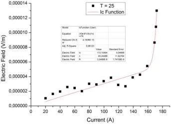
2.3 Measurements Ic

(16)

[image:16.595.104.448.83.335.2]

Figure 2.8: Graph of a critical current measurement at T = 25 K and B = 14 T.

the 2 mm wide tape, the sample got damaged. It must be noted that REBCO coated conduc-tors are relatively fragile and still in development: the quality of the REBCO is not uniform along its length. The tape was damaged at a weak point outside the zone monitored by the voltage taps. Also the temperature could not be controlled during the ramping of the current towards the critical point.

It was therefore decided to conduct the measurements of the critical current with a standard Ic-setup available in the superconductivity lab. This setup uses a simple custom-made program

called 'VI', which monitors several volt meters. Also the current and magnetic eld can be controlled from this program. Three voltage pairs soldered on the tape, measuring over the whole tape length, over a length outside the heaters and inside the heaters. Also a Cryocon temperature controller can be used with this setup. The controller monitors the thermometers and control the edge heaters to tune the temperature. Especially near the critical current, maintaining the temperature is of importance, since ohmic heating at the soldered current leads can raise the temperature of the whole sample. The temperature controller also has internal relays that can be used to interrupt the current control signal. These relays can be set to open the circuit at a maximum temperature. In this way there is another safety measure. In spite of all the safety measures, the measurements of the critical current were dicult. The tape has a fast increasing critical current at temperatures lower than 23 K, even at the highest magnetic eld of 14 T. After the measurements on the 4-mm wide tape, the Lorentz forces were directed outwards. As discussed above, when these forces point inwards, the tape could buckle when it is not tightly wound around the structure or kink between the ridges. But in this conguration, with the Lorentz forces pointing outward, the hoop stresses became too high. The data that could be collected are represented in table 2.1. Figure 2.8 shows the current-electric eld curve registered during a critical current measurement at T = 25 K and B = 14 T. In appendix B, all the graphs of Ic-measurements can be found.

(17)

[image:17.595.209.389.81.192.2]

Table 2.1: Critical current values found at a background magnetic eld of 14 T.

the Ic-measurements were considered too risky. The values are not of main importance for the

analysis of the M QE and Vnzp and could be determined after the NZP measurements. More

discussion aboutIc-values of the 2- and 4-mm wide tapes can be found in the Analysis, chapter

4 on page 26.

2.4 Measurements Vnzp

In this section, the dierent functional elements of the equipment schematically shown in gure 2.6 are discussed.

Current and magnetic eld controlThe experiment starts with the creation of a controlled environment. The EMS-laboratory has a 60 mm bore diameter, helium-cooled N b3Sn magnet

able to generate a maximum magnetic eld with a strength of 14 Tesla, powered by a Cryogenics power supply and controlled remotely with the 'VI'-program. The current through the sample is provided by a Delta SM 15-400 power supply able to deliver currents up to 400 A. Another supply was available capable of delivering 200 A, the Delta SM 15-200D. The sample current is measured with a Hitec Zero Flux probe, giving a signal of 0.005 V/A and able to measure currents up to 2000 A. The current is directly controlled by the DAQ 1 device. To stabilize the current control signal, a instrument amplier is used between the DAQ and the quench detector. The sample current is monitored with an accurate micro-volt meter to verify the correct registration by the DAQ 2 device. The critical current of the N b3Sn current leads is

440 A. As discussed earlier, because of this limit, it was decided to use a REBCO tape of 2 mm width.

Temperature control An important part is the control of the temperature. The experiment has to be performed as adiabatic as possible. The sample holder is lowered in a liquid helium bath of 4.2 K. The sample environment is vacuum-pumped to prevent unwanted heat loss to the bath by conduction or convection. It is pumped for at least two nights to a pressure below 0.01 Pa, using a Pfeier Hi-Cube pump. To check for leaks, the pressure is veried to increase no more than 1.8 Pa/h, presumably mainly due to out-gassing. When lowered in the liquid helium bath, any residual gas will freeze to the wall. This cryo-pumping ensures a good vacuum: in between measurements at room temperature, a small leak was discovered, but lowered in the cryostat the pressure in the vacuum chamber did not increase. To thermally insulate from the sample further, all electrical wiring is made of manganin wire with a diameter of 0.1 mm. There are three parts of thermal loss which cannot be prevented:

1. Thermal conduction to the nylon ridges on the sample support structure (gure 2.3 and 2.5)

(18)

T=4.2K

3. Thermal radiation from the tape to the support structure with the embedded heater The temperature is raised by three elements. In the support structure of the tape is the embedded heater. A resistive phosphor bronze heater wire runs along its whole length and thereby ensures an even spread of the heat. Its current is provided by a Delta E030-1 power supply in voltage mode. After adjusting the output of this embedded heater, it takes quite a long time for the temperature to stabilize, typically more than 240 seconds. This conrms the heat is spread gradually and that heat from the sample will not ow fast to the support structure when the temperature of the sample is raised during a quench. Most heat is conducted longitudinal through the tape towards the copper terminals of 4.2 K. Because of that, there are two edge heaters. These thick lm SMD resistors of 20Ω are attached at the ends of the tape and isolate the measured zone from the heat sink. The edge heaters allow accurate adjustment of the temperature and are powered by two Delta CST 100 current sources. The temperature is monitored with calibrated Cernox temperature sensors from Lake Shore Inc. and their power is supplied by a Lake Shore 121 current source. For all experiments, the X31553 and X78396 thermometers were used. The registration of the temperature is done by the DAQ 1 device, which features 18-bit input sampling and is thus more accurate than DAQ 2.

Quench initiation and registration When the temperature-, magnetic eld- and current environment of the sample is controlled and stabilized, the quench can be initiated. The heat is applied by a SMD resistor of 15Ω attached to the tape, as shown in gure 2.3. The current is supplied by a Bipolar Operational Source / Sink (BOS/S) amplier. This supply is set to amplify the controlling signal voltage from the DAQ 2 device by a factor of two. The maximum output of the amplier is 20 V and 20 A. The quench heater signal is a single square pulse, with a maximum height and width that can be adjusted in the Labview environment. The signal-registering device DAQ 1 has a voltage limit of only 10 V. To be able to measure a full signal, the voltage is divided with two 28 kΩresistances in series and later multiplied again in the software environment. When the quench heater warms up, its resistance will change. So the current through the quench heater is monitored separately by measuring the voltage over an accurate 0.1Ωshunt resistor. The energy of the pulse through the heater is then determined by the integral of the voltage and current over the time length of the pulse:

Epulse =

Z ∞

0

U ·Idt, (2.1)

where U is the voltage over the heater and I is the current through it.

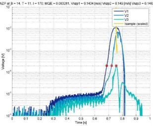
When the heat pulse is triggered, also the possible normal zone propagation is registered by the monitoring voltage taps on one side of the quench heater. The signal has to be measured fast and accurately, so each voltage pair signal is pre-amplied by an Ectron 751ELN DC-Amplier. The ampliers are set on a gain of 1000x and a low-pass lter bandwidth of 10 Hz. A smaller bandwidth (1 Hz) would slow down the signal-processing too much. The DAQ 2 device is used for the registration of the voltages. It has a sample rate of 10 kHz divided over three channels, which is higher than the DAQ 1 device. The voltage signal measured by the data acquisition card is divided by the voltage tap distance in the software, to produce the electric eld. The energy of the pulse then gradually increased until a quench occurs. A clear trace of measured voltage response during a quench is shown in gure 2.9.

(19)

current control signal or enabling the quench detection port of the power supplies. As discussed earlier, also the current leads of the insert are protected with this method. Besides the quench detection hardware, a software-based quench detection method is implemented for redundancy: if the signal of the voltage taps exceeds a certain trigger level, the current is set to zero. The current is also disabled automatically when a certain interval after a heat pulse has past. The quench detection has to respond quickly. Hardware detection is the most direct method and therefore, most of the time, the rst one to trigger. The device needs to be 'tuned' carefully: if the current is shut o too soon, the voltage signal of the quench is too small and unstable and the data are useless. After a rst sample burned out despite these redundant safety measures, a second quench detector was added to the setup to have more control.

Based on his experience with 4-mm wide tapes, J. van Nugteren [9] recommended to set the alarm level of the quench detector in such a way, that after a quench the temperature will not rise above 70 K at T1 and T2. For measurements on the 2-mm wide tape, this limit implied an alarm level of the quench detector which was too low for acquiring a clear voltage signal, i.e. the quench detector responded too quickly. The alarm level was raised until a usable voltage development could be measured. The corresponding maximum temperatures during a quench now lie around 110 K.

Software The NZP-experiment is mainly controlled with a Labview by written by J. van Nugteren [9]. Labview is a graphical programming environment developed by National Instru-ments. The Labview environment for NZP-experiment consists of several functional sections:

1. Environment control; monitor temperature and magnetic eld.

2. Ic-measurement and current control; monitor and control the sample current, ramp rate

and the voltages. An Ic-measurement can be started, slowly ramping from a starting

current and measuring the voltage until a certain level has been reached. Then the Ic

-measurement is terminated and the current is shut down.

3. Pulse response; set the pulse energy and monitor the outcome after a pulse. 4. Quench detection; settings for the software quench detection.

5. Data I/O; export the data from the last action (Ic-measurement or pulse response) as a

matlab-le.

6. Settings; indicators and controls of e.g. sampling frequencies, time, amplication, scaling and osets for components.

2.5 Signal analysis

(20)

[image:20.595.140.450.63.318.2]

Figure 2.9: A clear voltage signal from a quench event.

A quench is recognized as an exponential voltage level growth, which is shifted in time for the subsequent voltage pairs. Disturbances in the voltage prole are seen in gure 2.9, after t = 0.65 s at V2 and after t = 0.7 s at V3. These disturbances are seen in almost every measurement on 2-mm tape, in contrary to measurements on 4-mm tape. Because of these irregularities, the value ofVnzpis harder to determine. Therefore, of every measurement, (Vnzp, Vthreshold)a prole

like the one in gure 2.10 was determined by calculating Vnzp at dierent threshold voltages.

With such proles, a threshold voltage could be determined at which the propagation velocities are most stable and comparable with each other. This general threshold voltage was set at 0.2 mV. For a few measurements, the threshold voltages had to be adjusted slightly. The general threshold voltage used for 4-mm tape results was 0.1 mV, so the results stay comparable. The proles are also used to estimate uncertainties on the normal zone propagation velocities. A further possible source of errors is the inuence of the solder of the voltage taps. The voltage taps need to be soldered to the tape, as shown in gure 2.11. Care was taken to do this as 'cleanly' as possible, but a minimum amount of solder is needed for good contact. This solder adds material and thus heat capacity locally. The increase of heat capacity lowers the Vnzp, see

(21)

Figure 2.10: A prole of gure 2.9 withVnzpversus threshold voltage. At a threshold voltage of 200

[image:21.595.140.450.143.396.2]

µV, the signals are stable and the velocities of all taps are comparable.

(22)

Chapter 3 Results

In this chapter the results of the measurements on the 2-mm REBCO tapes are presented. The chapter starts with an overview of the experimental campaign. Next, the results of the minimum quench energy are presented as functions of temperature and current. Finally, also the normal zone propagation velocities are shown at various magnetic elds, temperatures and current levels.

3.1 Overview

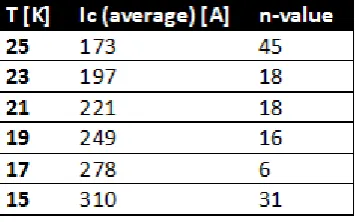
At the start of the assignment to measure MQE and Vnzp on 2-mm tapes and as discussed

in chapter 2, the electrical wiring was replaced. To test the modied set-up and to gain experience with the experiments, a new 4-mm REBCO tape was mounted. During a rst test run with this new 4-mm tape in the 15 T magnet, the embedded heater leads burned out and needed to be replaced with slightly thicker manganin wire. A successful set of experiments was then performed on the 4-mm tape, reproducibly yielding comparable Ic, MQE and Vnzp

data as those reported previously by J. van Nugteren [9]. During on of the Ic-measurements,

the sample broke at the quench heater, outside the monitored area. An extra voltage tap across the whole tape was added from this moment onward. Enough experience with the setup and the instrumentation was gained after this test run to commence the measurements on the 2-mm tapes. The heater elements were replaced with smaller versions from the same manufacturer and type. A Cryocon temperature controller was used to maintain a constant temperature during theIc-measurement. A set of successfulIc-measurements was conducted for

temperatures between 25 K to 19 K. At 19 K, the tape quenched and was damaged. Subsequent inspection revealed an overheated spot, once more outside the sample length monitored by the voltage taps. A new tape was prepared and three new voltage taps were added for Ic

-measurements. Apart from an initial (solved) grounding problem with a temperature sensor, the second Ic-measurement run gave good results. The addition of three voltage taps (V0,V4,V5)

for measuring Ic proved valuable. Six Ic-values were acquired at a magnetic eld strength of

14 T within the temperature range of 25 K and 15 K. Unfortunately however, at T = 13 K, the tape was pulled from the bottom terminal by the outward pointing Lorentz forces and the sample was destroyed. A picture of this tape can be seen in gure 3.1. Therefore, the third sample was reinforced with niobium titanium wire around the terminals. The outcome of the measurement can also be seen in gure 3.1: this time the sample burned through after one Ic

-value measurement, outside of the zone heated by the edge heaters. After this failed attempt to collect further Ic values at lower temperatures, it was decided to start the NZP measurements

and postpone theIc-measurements, to minimize the risk of damaging the tape. It was reasoned

that previous measurements could be used as a rst indication and after a successful NZP measurement run, theIccould still be determined. The fourth 2-mm wide sample burned right

(23)

approach, the fth sample nally gave adequate MQE and Vnzp results. These are presented in

the following sections.

(a)The second 2 mm wide sample (b) The third, burned out sample

Figure 3.1: Photographs of the sample after failed experiments. (a) This sample was electro-magnetically pulled from one of the soldered current terminals. (b) The tape burned out between the edge heater and the corresponding current terminal.

3.2 Mimimum Quench Energy

Although the focus of this assignment was on the determination of the normal propagation velocity, the experiments also yielded an estimate of the MQE-value under various operational parameters. As shown in gures 3.2 and 3.3, the MQE decreases with increasing temperature and current. Referring to equation 1.1, the temperature dependence of MQE is determined by two eects. A higher operating temperature T0 implies that the sample needs to be heated

less to reach the transition temperature Tt, so MQE goes down. The dierence Tt − T0 is

called the thermal margin. On the other hand, the heat capacity C(T)is a strongly increasing function of temperature. Based on this observation, MQE might be expected to go up with temperature. In the dissertation of H. van Weeren [8], it is mentioned that in M gB2 wires,

for which the set-up was originally designed and used, there is a competition between these two eects, leading to a non-monotonic temperature dependence of MQE. The thermal margin clearly has more inuence here in these REBCO tapes. Concerning the current dependence of MQE (gure 3.3), for a given magnetic eld, a higher sample current implies a lowerTt. So also

the observed decrease of MQE with increasing sample current can be interpreted as a decrease of the thermal margin. The dependence of MQE on magnetic eld, however, is anomalous. It may be expected that MQE decreases with increasing magnetic elds: for a given current Tt

and hence also the thermal margin will go down as the eld goes up. The measurements at a magnetic eld of 10 T from 15 K and lower temperatures, and the measurements at a magnetic eld of 14 T were made with a dierent quench heater xation. As discussed in section 2.1, the quench heater was glued to the tape with aluminum loaded epoxy, but detached several times and the xation had to be replaced. Therefore it is rather dicult to make conclusions on the dependence of the MQE on the magnetic eld.

(24)

Figure 3.2: The dependence of the MQE on temperature and magnetic eld, measured at a constant current of 170 A. The numbers are not adjusted for heater ineciency.

energy simply heats up the heater-leads. Moreover, the heater itself has a nite heat capacity and its thermal connection to the tape has a nite thermal impedance. This implies that when the heater and the thermal connection warms up, energy only gradually seeps in the sample. As a consequence, before the quench, some heat already can be lost to the environment because of radiation and the electrical connections of the heater. As a further complication, when the sample becomes normal, ohmic heat increases the samples temperature and part of this ohmic heating can ow back into the heater. All these eects make MQE measurements notoriously dicult to interpret [9].

3.3 Normal zone propagation velocity

In this section, we turn our attention to the measured normal zone propagation velocity (Vnzp).

The main goal of this assignment was to asses whether the conclusion of earlier work in the temperature range 25-45 K (i.e. the observation that Vnzp hardly depends on magnetic eld or

temperature) also extends to lower temperatures.

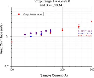
Figure 3.4 shows a total of 38 points measured at temperatures varying between 4.2 and 29 K, at a constant current of 170 A and at three dierent magnetic eld strengths (6, 10 and 14 T). Clearly the variation of the normal zone propagation velocity in this temperature- and eld range is hardly signicant. Several velocities, measured at the same temperature, but dierent magnetic eld strenghts, show an overlap. Note that the error estimates indicated in the gure were determined from the analysis of the threshold voltages, see section 2.5. A linear t through the points (gure 3.5) gives a slope of (5.3±1.7)×10−4 m/s per Kelvin in the

temperature range of 4.2 K to 29 K, i.e. the ttedVnzp variation over this range (∼1cm/s) is

of the same order as the typical uncertainty estimate on the Vnzp values (∼1−2 cm/s). Four

(25)

Figure 3.3: MQE versus sample current. The values of MQE are not compensated for any heater ineciencies.

Figure 3.4: Vnzp versus temperature. The velocity changes with 9 percent between 4.2 and 29 K. At several temperatures, the velocity at dierent magnetic eld strenghts show an overlap. The error was determined by analysing the threshold voltage (section 2.5)

(26)

These measurements were conducted in the beginning of the measurement period, at the start of the 'learning curve' described by the overview in section 3.1. The threshold voltages of the measurements were too low, because of a too tightly set quench detector. The quench detector cut o the current before a usable signal could develop.

Figure 3.5: The temperature dependence of Vnzp at a constant current of 170 A. A tted linear trend line is added, with a slope of(5.3±1.7)×10−4 m/s per Kelvin. Four points fell out of the error

margin and were excluded.

(27)

[image:27.595.126.452.269.538.2]

Figure 3.6: Vnzp measured versus sample current at three dierent combinations of magnetic eld

(28)

Chapter 4 Analysis

The theoretical description of normal zone propagation in low-temperature superconductors is based on the analysis of the heat balance equation, as described in of this chapter. Whether or not this 'classical' model can just as well be used for the REBCO HTS, is also explored in this rst section. In parallel with the experiments, numerical simulations were executed. The main conclusions of these simulations are summarized in section two. In the nal section, the data for the 2 mm wide tapes are compared with the previous observations on 4-mm REBCO tape.

4.1 Analytical model

The model of normal zone behavior is based on the heat balance equation. The one-dimensional version of this heat balance equation is given below (Eqn. 4.1).

C(T)∂T ∂t =

∂ ∂x

k(T)∂T ∂x

+PΩ+Pi −Pc (4.1)

Here C(T) is the temperature-dependent heat capacity in J/mK, k(T) the temperature de-pendent thermal conductivity in W m/K and T the temperature. The power terms PΩ, Pi and

Pc represent the Ohmic power dissipation in the tape, the initial disturbance and the cooling

to the environment respectively, all given in W/m. Assuming an adiabatic environment and a steady-state propagation of the normal zone (i.e. its propagation once transients due to the initial disturbance have died out),Pc and Pi are neglected, respectively. The diculty in

solv-ing the resultsolv-ing dierential equation lies in the non-linear character of the remainsolv-ing power term PΩ, which is caused by the non-linear electric eld - current density relation (see section

2.3). However, under some simplifying assumptions, the equation may be solved analytically at the interface between the normal zone and the superconducting parts of the sample to yield equation 4.2 for Vnzp. For the full derivation, see [7] or [9].

Vnzp=

Iop

C( ˜T) s

ρ( ˜T)k( ˜T) (Tt−Top)

. (4.2)

In this analytic expression of Vnzp, Iop is the current in the sample, C its heat capacity

(aver-aged over all constituent materials), ρ its average electrical resistivity in the normal state, k its average thermal conductivity, Tt the transition temperature and Top the operational base

temperature. With the simplications commonly made, the material-dependent properties are usually evaluated at an average temperature: _T˜_{= (}_T_t₊_T_op₎_/₂_.

(29)

temperatures. As a rst observation, the temperature range under consideration with HTS is obviously larger than for LTS. For the latter materials, the transition temperatureTt(depending

on current and magnetic eld) typically lies below 10 K while their operational temperature typically is 4.2 K. Here, Tt may be as high as 40 K and considering the material properties to

be constant is a crude approximation. The temperature dependence of the material properties is shown in gure 4.1. Crudely speaking all values drop with temperature, with the electrical resistivity becoming almost constant below 25 K and the heat capacity below 15 K. The thermal conductivity becomes linear below 15 K.

Figure 4.1: Calculated average material properties for the 2-mm wide REBCO tape [9]. Plotted against temperature are the electrical resistivity 'ρ', the thermal conductivity 'k' and the heat capacity

'C'.

In the book on superconducting magnet design by Iwasa [7], it is argued that the approximation of _T˜ _{should only be used if} ₍_T

t−Top)/Top 1. This is generally more or less applicable for

LTS materials, but in general not for HTS. Instead of equation 4.2, Iwasa suggests using a more exact version with temperature dependent material properties, proposed by Whetstone and Roos [11]:

Vnzp=I

v u u u u t

ρ(Tt)k(Tt)

C(Tt)−

1 k(Tt)

dk dT Tt

Z Tt

Top

C(T)dT #

Z Tt

Top

C(T)dT

(4.3)

We will refer to the prediction Eqn. 4.2 as the 'short model' and to Eqn. 4.3 as the 'long model'. The short model evaluates the material properties at a temperature which is too high, yielding temperature dependent Vnzp values. The long model considers the full temperature

range for the material properties and yields a Vnzp that is nearly temperature independent

below 25 K, conrming the experimental observations on the 2- and 4-mm wide REBCO tapes. Quantitatively, the long model prediction deviates about 15% from the 4 mm data and 33% from the 2 mm data. It should be noted, however, that the long model considers a fully adiabatic system, whereas the experiments are performed quasi-adiabatic (see section 2.4). Equation 4.3 shows that the predicted inuence of the current is seems to be linear, in contrast to the power close to 1.5 observed experimentally. We will refer further discussion of this discrepancy to the next section, where more precise theoretical predictions will be made based on a purely numerical model.

The last parameter that remains is the applied magnetic eld. An applied eld will mostly inuence the electrical resistivity, raising it. However, below 25 K the electrical resistivity is small and constant, so a magnetic eld is not expected to change the value of Vnzp to a great

(30)

[image:30.595.112.455.80.339.2]

Figure 4.2: Comparison of the 'short model' prediction Eqn. 4.2, the 'long model' prediction Eqn. 4.3, the 'power law' behavior observed in the 4 mm tapes [JvN] and the present data on the 2-mm tape. The models are considered at an operating current of 173 A and a magnetic eld of 14 T.

Another important analytical approximation which requires a closer look, is the choice of the transition temperature. It is dened as

Tt= (Tcs+Tc)/2 (4.4)

with Tcs the 'current sharing' temperature, i.e. the temperature at which the sample current

becomes equal to the (temperature dependent) critical current and the rst ohmic dissipation sets in. The choice of Tt midway the current sharing- and critical temerature was proposed by

Dresner [12]. It is based on a piece-wise solution of the heat balance equation to simplify the treatment of the current sharing regime. To clarify this concept, we consider the example in gure 4.3, where we indicate which fraction of the current is carried by the REBCO layer of the tape and which fraction ows in the copper stabilizer (see also gure 2.1). Three regions are distinguished:

• Fully superconducting - In gure 4.3, below Tcs = 30 K. All current is owing through

the superconductor and there is no Ohmic heating.

• Current sharing - In gure 4.3, between Tcs K and Tc = 68 K. The Ic drops below the

operating current, forcing a part of it through the normal conductor, generating heat.

• Fully normal - In gure 4.3, aboveTc= 68, all superconductivity is lost.

Matching the solutions for all three regimes at the boundaries, creates an implicit equation which can not be written in a closed analytic form. Therefore, Dresner proposed to treat current sharing with the more simple step function of equation 4.4, which does lead to a closed analytic expression. By doing this, he assumes that below Tt all current ows loss-less

in the superconductor, while above Tt the full current ows in the stabilizer. However, the

(31)

[image:31.595.160.431.133.347.2]

cruder. Constructing an alternative analytical prediction that avoids this central current sharing simplication is a task that was considered to lie outside the scope of this MSc assignment, especially since nowadays relatively straightforward numerical models can be constructed and evaluated. Such a model is the topic of the next section.

Figure 4.3: Example of current sharing in the 4-mm tape. Tcs is at T = 30 K. Tcis at T = 68 K.

4.2 Simulations

In parallel with the NZP experiments on the 2-mm wide HTS tape, simulations were conducted to support the ndings of the experiments, in the same manner as was done for the 4-mm tape. The simulations for the 2-mm tape were executed by Remco Timmer in the frame of his BSc assignment and solves of the discrete heat balance equation in a one-dimensional lumped system.

C(Ti)

dTi

dt =

k(Ti)(2Ti−Ti−1−Ti+1)

dxi

+I_nc2 ρ(Ti)dxi+Pi(xi, t)−h(Ti−Top)dxi. (4.5)

Once more C(T)is the temperature-dependent heat capacity inJ/mK,k(T)the temperature-dependent thermal conductivity W m/K,ρ(T)the temperature-dependent electrical resistivity in Ω/m and dxi the length of the node with index i.

Solving the heat equation numerically, the slow transition of the HTS shown in gure 4.3 can be fully incorporated. Also the temperature dependence of the material properties can be fully taken into account. The discrete form of the heat equation is solved using Matlab ode15s dierential equation solver. A sample length of 0.2 m is divided in a number of nodes and all nodes are attributed the same temperature Top at the start. The quench is initiated

at the center node by the disturbance term Pi. An example of the resulting evolution of the

temperature prole is shown in gure 4.4.

For the description of the current sharing regime (4.3) and the corresponding calculation of the power dissipation term PΩ, the temperature- and magnetic eld dependent critical current

values of the tape are required. However, a full description of the critical surface (see 1.2) of these tapes was not available and the experimental campaign to determineIcbelow 25 K proved

(32)

[image:32.595.136.452.72.345.2]

Figure 4.4: Temperature development of a simulated quench, with B = 14T at T = 4.2 K and I = 170 A.

this lowest temperature range. Two types of scaling relations were investigated: an exponential scaling relation, proposed by C. Senatore [13] and a bi-linear scaling. Earlier measurements of V. Lombardo [14] and J. van Nugteren indicate a bi-linear relation, i.e. scaling with two seperate linear ttings with a transition from one to the other between 30 K and 40 K. In gure 4.5, the measured Ic values and the investigated scaling relations are shown. Both scaling relations

approach the available measurements fairly well.

With these extrapolated critical current values, simulations were performed and the results were compared with the measurements. The results for the temperature dependence of Vnzp is

presented in gure 4.6 and the current dependence in gure 4.7. The temperature-independent value for the 4 mm wide tape [9] is shown together with the measurements done on the 2-mm wide tape.

All solutions of the simulation lie below the power law and above the measurements on the 2 mm wide sample. Though the values dier from the measurements, the simulations conrm the limited dependence of Vnzp on magnetic eld and temperature. The simulations with the

bi-linear current-temperature relation yield values that are about 25% higher than the points calculated using the exponential scaling relation. The bi-linear scaling is more realistic because theIcvalues do not 'explode' at low temperatures. However, the exponential readings are more

(33)

[image:33.595.90.488.97.338.2]

Figure 4.5: Critical current density values at dierent magnetic eld strengths, used for the simu-lations. The points represent the measured values, the lines show the values using the tted scaling relations. JvN stands for the measurements of the 4-mm wide tape, BH for the 2-mm wide tape data collected in this work. Behind the name in the legend the value of the magnetic background eld is indicated.

Figure 4.6: Results from the simulation of temperature dependence ofVnzp, at a constant current of

[image:33.595.99.523.495.717.2]

(34)

[image:34.595.97.527.71.285.2]

Figure 4.7: Results from the simulation of current dependent Vnzp. For T = 4.2 K at B = 6 T; T =

25 K at B = 10 T and T = 23 K at B = 14 T.

4.3 Comparison of normal zone propagation in the 2 - and 4 mm wide

tapes

One of the goals of the research in this report was to verify the power-law dependence of the normal zone propagation velocity on the sample operating current. In gure 4.8, the normal zone propagation velocity against the current is tted with a exponential function:

Vnzp= 10P2IP1 (4.6)

The power-law behavior found by J. van Nugteren [9] is also drawn as a solid light grey line. Comparison of the tted power-law Eqn. 4.6 shows a great similarity in the slope, but there is a rather large dierence in Vnzp values, with the propagation in the 2 mm wide tape40−50 %

lower than in the 4 mm wide one. In table 4.1 the coecientsP1 and P2 are summarized.

Table 4.1: Fitting coecients P1 and P2 of equation 4.6 for the two HTS samples

4.3.1 Possible causes for the dierences between the 2-mm and 4-mm tape

Although the temperature-, magnetic eld - and current dependence ofVnzp is similar for both

tape widths, the absolute dierence between theVnzpvalues measured in both tapes is relatively

large. In the following subsection probable causes for this dierence are further explored.

Copper layer thicknessAs discussed in section 2.1, a large part of the REBCO tape consists of copper stabilizer. According to equation 4.2, the copper inuences the value of Vnzp directly

(35)

Figure 4.8: Measured Vnzpcompared with the earlier found current dependence

the thermal and electrical properties of the tape. Moreover, the copper layer is electroplated and its thickness is less controlled than the other material layers. Cross-sections of the 4-mm and 2-mm wide tape were polished and images were taken, as shown in gure 4.9 and 4.10. Due to electrostatic edge eects during the copper deposition, a buildup of copper is seen near the edges of both tapes, a phenomenon that in the community is commonly called 'dogbone shape'. This thickness inaccuracy is inherent with the electroplating technique. Because of its smaller dimensions, the inuence of this copper accumulation at the edges might have a relatively large eect on the properties of the 2-mm tape. To check whether the conductors have a signicantly dierent relative amount of copper, these cross-sectional images were analyzed in detail. The conclusion is that the 2-mm wide tape has (7±1)% more copper than the 4-mm wide tape. With the numerical model described in section 4.2, it was concluded that this leads to a decrease of Vnzp with almost the same percentage: (8±1)%.

[image:35.595.98.489.61.359.2]

Figure 4.9: Cross section of the 2-mm tape. Notice 'dog bone' shape of the tape, i.e. the increased amount of copper at the edges.

Figure 4.10: Crossection of the 4-mm tape used for measurements executed by J. van Nugteren [9].

Width of the tape To compare the 2-mm to the 4-mm tape, the values of the Ic, Vnzp and

(36)

tapes need to be measured accurately. Once more using the cross-sectional images in gure 4.9 and 4.10, the widths of the tape were determined with a higher precision. The widths were found to be (2.01±0.01) mm and (4.02±0.01) mm respectively. These values includes the irregular shaped copper layer. The width of the REBCO layer itself is (1.93±0.01) mm and (3.97±0.01). The scaling factor should therefore be 2.06. This would imply the current densities would go up by 3%, in the comparison to theIcvalues reported in gure 4.5. Assuming

that the 2-mm tape has a comparable quality as the 4-mm tape. The rescaling of values would imply a lowerVnzp with the same factor as the current. In other words, the 2-mm values would

fall an extra3% with respect to the 4 mm ones. This correction is minor and, moreover, in the wrong direction to explain the observed Vnzp dierence.

Minimum propagation zone To register a steady-state propagation velocity, the voltage taps need to be located suciently far from the quench starting point. A crude rst estimate indicates that the minimum distance is about equal to the minimum propagation zone length `M P Z (see section 1.3). Vnzp is supposed to become stable once it has propagated beyond the

M P Z. Using equation 1.1 on page 4, the`M P Z is calculated. At 25 K, theM P Z is estimated

to have a length of 0.47 mm and at 4.2 K it has an even smaller length of 0.26 mm. So Vnzp

should be stable at the voltage taps, which are placed 10, 15 and 20 mm away from the quench initiation heater.

Cooling term The heat balance equation 4.1 contains a cooling term Pc, which takes into

account heat leaking away from the normal zone to the environment and consists of a radiation part and a conduction part to the support structure. The cooling term could give an indication for dierence between the two tapes. Increased cooling during a quench results in a lower amount of heat available to drive the superconducting-to-normal front forwards and hence to a lower propagation velocity. Estimating the radiation part yields 0.012W/m, which is negligible compared to conduction losses. Analyzing the conduction term at 25 K and 4.2 K for the 2-mm tape gives a cooling factor of 2.3 W/m at 25 K and 1.8 W/m at 4.2 K, respectively. These values are smaller for the 2-mm than the 4-mm, so they cannot explain the lowerVnzp value in

the narrower tape.

The most plausible causes for the observedVnzp dierences between the 2-mm and 4-mm wide

(37)

Chapter 5 Discussion and conclusion

The normal zone propagation velocity and minimum quench energy of a 2 mm wide REBCO coated conductor tape were measured at magnetic eld strengths of 6, 10 and 14 Tesla. The measurements were successfully conducted as a function of temperature in the range of 4.2 K to 25 K at a constant current of 170 A. The velocity and quench energy were also investigated as a function of current with the temperature held constant at 4.2 K, 23 K and 25 K.

The minimum quench energy was found to decrease with increasing sample current, as might be expected from theory: when the current is raised the transition temperature goes down and the thermal margin, that needs to be overcome to turn the sample normal, becomes smaller. A similar eect was found in the temperature dependence of MQE. Raising the temperature at xed current also decreases the thermal margin and hence reduces the amount of heat needed to drive the tape into the normal state. Note that - unlike the current dependence - this conclusion for the temperature dependence of MQE is non-trivial. Theory as well as earlier observations on M gB2 wires show that the reduced thermal margin needs to be balanced against an increased

heat capacity, which might induce the opposite temperature dependence. However, just like in earlier observations on 4-mm wide tapes, the data on the 2-mm wide samples show that the eect of thermal margin reduction dominates. Unfortunately, after a rst measurement series at relatively high temperature in a magnetic eld of 6 T, problems with the quench heater required a dierent way of attaching it to the tape, inuencing the measurements of MQE at the lower temperatures of 14 T and 10 T. Therefore, no hard conclusions can be drawn on the magnetic eld dependence of the MQE.

It was shown that the normal zone propagation velocity is almost independent of the tempera-ture, with a barely signicant increase of 9% between 4.2 K and 29 K. Also the magnetic eld strength hardly seems to have an inuence on the Vnzp at xed temperature and current for

elds between 6 T and 14 T.

The analytic model based on the heat balance equation with the approximation of Dresner was compared to the measured data. The model predicts a temperature dependence ofVnzp due to

the temperature dependence of the materials properties: heat conduction, electrical resistivity and heat capacity. For low temperature superconductors, these can be evaluated at an average temperature. However, as pointed out by Iwasa, this type of averaging becomes incorrect for high temperature superconductors and a more exact model was used, which integrates the full temperature dependence of the material properties over the whole temperature range of interest. It was shown this type of model indeed predicts the observed temperature independence ofVnzp

below T = 25 K.

To obtain a more detailed comparison with theory, numerical simulations were executed and their results were compared to the data. A scaling relation had to used for the critical current, because reliable Ic-values not could be obtained below T = 15 K for the 2-mm wide tape. The

Ic-values that were found at higher temperatures, are in good agreement with the Ic-values

(38)

the tape should be of similar quality. The simulations of the normal zone propagation using dierent scaling relations show some spread, but lie below theVnzpvalues measured in the 4-mm

tape and above those of the 2-mm tape. Both mainly depend on the operating current and only slightly on temperature. The magnetic eld seems to have more inuence in the simulations than in the measurements. Although the results are not fully comparable, the simple and computationally ecient numerical 1D-model gives a good insight in the Vnzp behavior.

One of the main goals of the assignment was to verify the dependence of the normal zone prop-agation velocity on the sample operating current. Earlier work on a 4 mm wide tape reported a power-law relationship between both, but could not be extended to lower temperature due to prohibitively large critical currents and associated high MQE values. Extending the mea-surements of the 4-mm tape at temperatures above 25 K to temperatures below 25 K, a good qualitative agreement was found between the current-dependence in both temperature regions. The power-law exponent is almost the same, but there is a 50% dierence in the absolute value of Vnzp observed in both tapes. At the writing of this report, the cause of the dierence in

(39)

Recommendations

The main goals of this master assignment are achieved, but some subjects can be investigated further. Also a lot of experience was gained during this measurement campaign. Therefore, some recommendation are given for improvements and future research.

• The 'RRR'-value of the copper layer was not determined accurately. Comparison of the

RRR-value of the 2-mm and 4-mm wide samples, could give further explanation for the quantitative dierences of their Vnzp-values.

• There were big dierences between the MQE value of the 2-mm and 4-mm wide samples.

The QE could inuence theVnzp. Registration of quenches at higher QE values is advised.

• The exact analytic equation 4.3 was only investigated qualitatively for the 2-mm wide

sample. Introducing a cooling factor make the model quantitatively more comparable.

• HTS coated conductors of other manufacturers exist. The NZP behavior of these tapes

can also be investigated and could give further insight in their behavior.

• When the NZP-experiments are continued using the existing setup, it is advised to

up-grade the current leads with HTS to handle higher currents and temperatures.

• During this measurement campaign, the results from the third voltage pair could not

used, because of an unclear signal. In this case, the rst two of the redundant voltage pairs should be used. Or all voltage pairs should be placed closer to the quench heater.

• The voltage taps for registering the Vnzp are not used for Ic-measurements. The second

end of theVnzp pairs should be placed at one point.

• During Ic-measurements, the sample should be fully wrapped with, for example kapton,

(40)

Acknowledgements

First, I would like to thank those who were directly involved with the work outlined in this thesis. Marc Dhallé, whom without this thesis wouldn't be as it is now, he has my full respect. For all the help in the lab, which was a lot, I would like to thank Sander Wessels. My

gratitude goes Marcel ter Brake, the professor of the EMS group where I am involved since my bachelor assignment. And Harold Zandvliet, as external committee member, being there

at the last moments of me being a student. Now I am sounding melancholic, however I am only grateful. There are so many I would like to thank for so many experiences during the years at this university. My family, for always being there and never giving me any doubt. My atmates, for lifting me up and putting me down. Friends and acquaintances at many places, like the study association Arago, sport association, the big band and so many in

between. I would like to thank my colleagues at EMS for the nice conversations and everything I can't think of. Thank you all for being there. Just let me nish with the words:

(41)

Nomenclature

This list gives a description of all symbols used in the report.

Symbol Description Unit

B Magnetic eld [T]

Bc1 First critical eld [T]

Bc2 Second or upper critical eld [T]

C One dimensional heat capacity [J/mK]

C0 Geometric average one dimensional heat capacity [J/mK]

E Electric eld [V /m]

E0 Electric eld used in the denition of the critical current [V /m]

Epulse Energy contained in a heater pulse [J]

h Heat transfer coecient for cooling to the environment [W/mK]

hcu Thickness (height) of the copper layer [m]

i Index of Node N.A.

Jc Critical current density [A/mm2

I Electrical current [A]

Iop Sample current [A]

Isample Sample current [A]

Inc Electrical current in the normal conducting parts of the sample [A]

Isc Electrical current in the superconducting parts of the sample [A]

k One dimensional thermal conductivity [W m/K]

M QE Minimal quench energy [J]

nnodes Total number of nodes N.A.

N N-value of a superconductor N.A.

PΩ Ohmic heating power [J/sm]

Pi Quench initialisation power [J/sm]

Pc Cooling power [J/sm]

QE Quench energy [J]

R Electrical resistance [Ω]

t Time [s]

tpulse Duration of a heat pulse [s]

T Temperature [K]

Tcs Current sharing temperature [K]

Tc Critical temperature [K]

Tt Transition temperature [K]

Top Operating temperature [K]

Ti Temperature of the node at index i [K]

˜

T Average temperature between Tt and Top [K]

(42)

Symbol Description Unit

Vnzp Normal zone propagation velocity [m/s]

U` Normal zone propagation velocity [m/s]

wsample Sample width [m]

x Spacial coordinate [m]

xi position of the node at index i [m]

ρ One dimensional electrical resistivity [Ω/m]

(43)

Bibliography

[1] H. Kamerlingh Onnes. Sur les Résistances Électriques. Communications from the Physical Laboratory of the University of Leiden, pages 111, 1911. Supplement 29.

[2] J.G. Bednorz and K.A. Müller. Possible high TC superconductivity in the Ba-La-Cu-O system. Zeitschrift für Physik B, 64(2):189193, 1986.

[3] H. Maeda, Y. Tanaka, M. Fukutumi, and T. Asano. A New High-Tc Oxide Superconductor Without a Rare Earth Element. Japanese Journal of Applied Physics, 27(2):L209L210, 1988.

[4] M.K. Wu, J.R. Ashburn, C.J. Torng, et al. Superconductivity at 93 K in a New Mixed-Phase Y-Ba-Cu-O Compound System at Ambient Pressure. Physical Review Letters, 58(9):908910, 1987.

[5] V.L. Ginzburg and E.A. Andryushin. Superconductivity. World Scientic, revised edition, 2004.

[6] M. Tinkham. Introduction to Superconductivity. Dover, second edition, 2004.

[7] Y. Iwasa. Case Studies in Superconducting Magnets. Springer Science, 2nd edition, 2009. [8] H. van Weeren.Magnesium Diboride Superconductors for Magnet Applications. PhD thesis,

University of Twente, 2007.

[9] J. van Nugteren. Normal Zone Propagation in a YBCO Superconducting Tape. Master's thesis, Twente University, 2012.

[10] D. Uglietti, H. Kitaguchi, S. Choi, and T. Kiyoshi. Angular Dependence of Critical Cur-rent in Coated Conductors at 4.2 K and Magnet Design. IEEE Transactions on Applied Superconductivity, 19(3):29092912, 2009.

[11] C.N. Whetstone and C.E. Roos. Thermal Phase Transitions in Superconducting Nb-Zr Alloys. Journal of Applied Physics, 36(3):783791, 1965.

[12] L. Dresner. Analytic Solution for the Propagation Velocity in Superconducting Composites. IEEE Transactions on Magnetics, 15(1):328330, January 1979.

[13] C. Senatore. Overview of the critical surface of industrial CC for EuCARD-2, 21-23 May 2014. 1st Workshop on Accelerator Magnets in HTS, Desy Hamburg.

(44)

(45)

Manual

of the

Normal Zone Propagation experiment

2014

(46)

1. Introduction ... 3

NZP and MQE ... 3 Setup ... 3 Design ... 3 Insert wiring ... 4 Sample holder... 5

2. Instrumentation ... 6

Connections ... 8 Quench detector sensitivity ... 11 Sample Preparation ... 12 Mount procedure ... 13 Testing ... 15 Closing up ... 15

3. Measurements protocols ... 16

Preparation - day before measurements ... 16 Preparation - day of measurements... 16 Normal zone propagation velocity measurements ... 16 During the measurements ... 17 Labview ... 17 Critical current measurements ... 17 Analyses ... 18