http://wrap.warwick.ac.uk
Original citation:
Leeke, Matthew, Arif, Saima, Jhumka, Arshad and Anand, Sarabjot Singh (2011) A
methodology for the generation of efficient error detection mechanisms. In: 2011
IEEE/IFIP 41st International Conference on Dependable Systems & Networks (DSN),
Hong Kong , 27-30 Jun 2011 . Published in: International Conference on Dependable
Systems and Networks. Proceedings pp. 25-36.
Permanent WRAP url:
http://wrap.warwick.ac.uk/42360
Copyright and reuse:
The Warwick Research Archive Portal (WRAP) makes this work by researchers of the
University of Warwick available open access under the following conditions. Copyright ©
and all moral rights to the version of the paper presented here belong to the individual
author(s) and/or other copyright owners. To the extent reasonable and practicable the
material made available in WRAP has been checked for eligibility before being made
available.
Copies of full items can be used for personal research or study, educational, or not-for
profit purposes without prior permission or charge. Provided that the authors, title and
full bibliographic details are credited, a hyperlink and/or URL is given for the original
metadata page and the content is not changed in any way.
Copyright statement:
“© 2011 IEEE. Personal use of this material is permitted. Permission from IEEE must be
obtained for all other uses, in any current or future media, including reprinting
/republishing this material for advertising or promotional purposes, creating new
collective works, for resale or redistribution to servers or lists, or reuse of any
copyrighted component of this work in other works.”
A note on versions:
The version presented here may differ from the published version or, version of record, if
you wish to cite this item you are advised to consult the publisher’s version. Please see
the ‘permanent WRAP url’ above for details on accessing the published version and note
that access may require a subscription.
A Methodology for the Generation of Efficient Error Detection Mechanisms
Matthew Leeke, Saima Arif, Arshad Jhumka and Sarabjot Singh Anand
Department of Computer Science University of Warwick Coventry, UK, CV4 7AL
{matt, saima, arshad, ssanand}@dcs.warwick.ac.uk
Abstract—A dependable software system must contain error
detection mechanisms and error recovery mechanisms. Soft-ware components for the detection of errors are typically designed based on a system specification or the experience of software engineers, with their efficiency typically being measured using fault injection and metrics such as coverage and latency. In this paper, we introduce a methodology for the design of highly efficient error detection mechanisms. The proposed methodology combines fault injection analysis and data mining techniques in order to generate predicates for efficient error detection mechanisms. The results presented demonstrate the viability of the methodology as an approach for the development of efficient error detection mechanisms, as the predicates generated yield a true positive rate of almost 100% and a false positive rate very close to 0% for the detection of failure-inducing states. The main advantage of the proposed methodology over current state-of-the-art approaches is that efficient detectors are obtained by design, rather than by using specification-based detectors or the experience of software engineers.
Keywords-Software Dependability; Fault Injection; Data
Min-ing; Error Detection Mechanisms; Decision Tree Induction
I. INTRODUCTION
The design of dependable software systems is known to be an inherently difficult problem [1]. A dependable software system must contain two types of dependability component, viz., error detection mechanisms and error recovery mech-anisms [2], which are commonly known as detectors and correctors respectively. A detector component is a program component that asserts the validity of a predicate in a program at a given location [2] [3]. To evaluate the effi-ciency of a detector component in a software system, fault injection is used to evaluate metrics [4], such as coverage and latency [5], that capture efficiency properties [6] [7]. If the values of these efficiency metrics do not reach a given threshold, the detector component under test must be redesigned or relocated and the efficiency metrics evaluated once more. This process is repeated until the efficiency prop-erties of the detector component satisfy the dependability requirements placed on the software system.
Detector components are currently designed based on a system specification [6] or the experience of software engineers [8]. It has been shown that the efficiency properties of detectors can be classified along two dimensions; (i) completeness and (ii) accuracy [3]. The completeness of a
detector component relates to its ability to detect erroneous states, i.e., to flag true positives, whilst accuracy relates to its ability to avoid making incorrect detections, i.e., to avoid false positives. An erroneous state is one that will lead to failure if the error is not handled. Failure is characterised as a violation of the system specification. A detector that is both complete and accurate is known as a perfect detector. However, due to implementation constraints, e.g., read/write restrictions, it is, in general, not possible to develop perfect detectors [9]. A perfect detector at a given location in a program is therefore the most efficient detector for that location. In this paper, we use the term efficient detector to refer to a detector with high completeness and high accuracy. Research that has addressed the systematic design of effi-cient detectors has generally focused on finite-state software systems [2] [3] [10] [11]. However, little work has focused on the systematic design of efficient detectors for real-world (infinite-state) software systems. In this paper, we address this problem through a novel methodology for the design of efficient detector components. Most significantly, the proposed methodology is applicable to infinite-state software systems and generates detector components whose efficiency is guaranteed by design. The premise of the methodology is that, given a program location at which a detector component will be located and for which the detector must be obtained, optimised data mining techniques can be used to analyse fault injection data in order to obtain efficient predicates for that detector component.
A. Contributions
In this paper, we make the following specific contributions:
• We propose a methodology for the generation of effi-cient predicates for detectors based on the application of data mining techniques to fault injection data. • We apply the proposed methodology to modules in
three complex software systems using the PROPANE tool [12] and the Weka Data Mining suite [13]. • We evaluate the effectiveness and complexity of the
The overarching contribution of this paper is to propose a data mining-based approach as an effective methodology for the generation of efficient error detection mechanisms. The generality of the proposed methodology is based on the premise that fault injection analysis performed under a known fault model can capture some relationship between the states of an executing program and the behaviours exhibited by that program. Typically fault injection data is interpreted with respect to the goal of understanding situations that lead to failure. The approach advocated in this paper takes this notion further, in that data mining algorithms are used to generate predicates which capture aspects of program correctness to be used in error detection mechanisms. The generated predicates are efficient, in the sense that they have a high accuracy and completeness.
B. Paper Structure
The remainder of this paper is structured as follows: In Section II we provide a survey of existing work in the area of detector design. We then detail the adopted system and fault models in Section III. In Section IV we provide background on data mining techniques that are relevant to the proposed methodology. In Section V we provide an overview of the methodology, as well as a description of each step required for its application. In Section VI we explain the experimental setup used to validate the proposed methodology. In Section VII we demonstrate the type of results the methodology is capable of generating. In Section VIII we discuss the main characteristics and limitations of the methodology, before concluding in Section IX with a paper summary and a discussion of future work.
II. RELATEDWORK
When designing a dependable software system, two impor-tant challenges exist, namely (i) the design of the depend-ability components, i.e, detectors and correctors, and (ii) the subsequent location/placement of these components [14] to contain the propagation of errors. Metrics, such as coverage and latency [5], are often used to evaluate the efficiency of dependability components. In general, coverage relates to the design problem, while latency relates to the location problem. In this paper, we focus on thedesignproblem and assume that the program locations are known, e.g., through techniques such as [14].
A. Detector Design
Several previous approaches to the detector design problem have focused on experimentally evaluating the coverage and latency of executable assertions (EAs) using fault injection. Through these approaches, it was established that EAs ex-hibiting high coverage and low latency serve to reduce error propagation. However, designing such EAs is difficult and error-prone, as demonstrated in [8], where it was remarked that “...the process of writing self checks is obviously
difficult”. To remedy this the authors in [8] suggested that “...more training or experience might be helpful”.
One approach for designing EAs uses the specification of a software system, or the constraints placed on its signals, i.e., parameters, to design corresponding EAs, e.g., [6] [7]. These EAs may not exhibit the high efficiency needed in dependable systems [15]. Specifically, it has been shown in [15] that such EAs may not flag erroneous states, i.e., false negatives, or may incorrectly flag correct states as being erroneous, i.e., false positives. When EAs do not meet the coverage threshold required of a system, they must be redesigned. However, very little work exists that helps with the refinement of EAs in practical software. The refinement of detectors has been investigated in finite-state systems, represented as state transition systems, e.g., [3] [11]. In these approaches, polynomial-time algorithms have been developed to automatically refine detectors. As a matter of contrast, we target the refinement of predicates for EAs for real-world (infinite state) software systems, through the use of data mining techniques. This problem has received very little attention in existing literature.
B. Data Mining Techniques
Data mining techniques have been used in the analysis of failure data for dependable software. For example, Pint´er
et.al [16] used data mining techniques on raw data obtained during dependability benchmarking to identify key infras-tructural factors for determining the behaviour of systems in the presence of faults. These investigations can help to identify weaknesses or vulnerabilities in a software system. As a matter of contrast, we propose a new approach, which complements existing ones, where by predicates for error detection mechanisms are discovered in order to limit error propagation, i.e, we develop detection mechanisms that ad-dress vulnerabilities. Data mining techniques have also been applied to address a number of other software dependability issues. For example, in the context of computer security, data mining has been shown to be an effective approach to intrusion detection and anomaly identification [17] [18].
C. Static Analysis
known to over-approximate the behaviours of a system. The abstract system is therefore made simpler to analyse at the expense of incompleteness, as not every property that is true of the original system is also true of the abstract system. However, if properly done, abstract interpretation is sound, meaning that every property that is true of the abstract system can be mapped to a property that is true of the original system.
It is well-known that, barring some hypothesis that the state space of programs is finite and small, finding all possible run-time errors, or more generally any kind of violation of a specification on the final result of a program, is undecidable. Thus, static analyses performed on a program are, in general, sound, in the sense that the properties they report are true.
D. Likely Program Invariants
An invariant is a property that holds at a certain point or points in a program. Determining all the sound invariants for a program may be undecidable. Further, invariants reported may not be sound, i.e., an invariant may hold true for most executions, but not for some. Thus, determining likely invari-ants [22] may be the best approximation, though steps must be taken to handle false positives. The use of invariants is valuable in many aspects of software development, including program design, implementation, testing and maintenance. Unfortunately, explicit invariants are usually absent from programs, depriving programmers and automated tools of their benefits. The seminal work on discovering likely pro-gram invariants [22] shows how invariants can be dynam-ically detected from program traces that capture variable values at program points of interest. The user runs the target program over a test suite to create the traces, and an invariant detector determines which properties and relationships hold over both explicit variables and other expressions. A tool, called Daikon, exists that supports the discovery of likely program invariants. Subsequently, several applications of the techniques have been proposed. For example, Demsky et.al [23] applied these techniques to discover invariants of abstract data types. More recently, these techniques have been applied to detect permanent hardware failures [24]. Dynamic invariant detection is a machine learning technique that can be applied to arbitrary data. However, invariants generally do not hold in presence of transient failures. Our approach differs from using Daikon as the tool has to be run in parallel with the software under test, i.e., it is an online approach, while our approach operates on data derived from fault injection, i.e., it is an offline approach. Moreover, our approach seeks to detect erroneous states that lead to failure rather than all erroneous states.
III. MODELS
In this section, we present the system model and fault model assumed by the analysis presented in this paper.
A. System Model
The methodology presented in this paper is concerned with the analysis and enhancement of modular software, thus we adopt a generic model of modular software systems. A software system S is considered to be a set of intercon-nected modules M1. . . Mn. A module Mk contains a set
of non-composite variables Vk and a sequence of actions
Ak1. . . Aki. The variables inVk have a specific domain of
values. Each action in Ak1. . . Aki may read or write to a
subset of variables inS
kVk.
In this paper we assume software to be grey box, meaning that access to source code is permitted, but knowledge of functionality and structure is not assumed, i.e., white box access with black box knowledge.
B. Fault model
We assume a transient data value fault model [25], which occurs when internal variables of a system hold erroneous values. The transient fault model is generally used to model hardware faults in which bit flips occur in memory areas that causes instantaneous changes to values held in memory.
IV. DATAMINING
Given a real-world process, great strides have been made with respect to the modelling, collection, storage and query-ing of data generated by the process. The process data is usually modelled by a set of entities, their attributes and their relationship to other entities. This is commonly known as the relational model of data. Data generated, and hence stored, within such a relational data model is a sample of all the data that may be generated by the process. Often, rather than being interested in the retrieval of stored data, we are more interested in forecasting behaviours of the process not previously encountered or learning some knowledge about the process if the process itself is not well understood. For example. we might be interested to learn how a software system may behave when faced with an injected fault.
Data mining aims to learn useful and actionable knowl-edge from large collections of data. In simple domains, it is not unusual to assume that the data is a single relation consisting of a set of n input attributes that define an n -dimensional space called the Instance Space,I. Every point inI is a potential state of the process being modelled. In supervised learning the data mining algorithm is tasked with learning a good approximation,fˆ, of an unknown functionf
(referred to as the target function) given a training data set,
T ⊆I, consisting of the N pairshxi, f(xi)i. If the function
Table I
CONFUSIONMATRIXEXAMPLE
Predicted Class Pos. Neg. Marginal Sum
Actual Class
Pos. TP FN npos
Neg. FP TN nneg
Marginal Sums nˆpos nˆneg n
positive instances as opposed to negative instances, which are instances that do not belong to the concept.
A number of algorithms have been proposed for classifica-tion, including Na¨ıve Bayes, nearest neighbour, support vec-tor machines (SVM), logistic regression, neural networks, decision tree induction and rule induction. They each differ in the kind of decision boundary they define between classes, i.e., their functional form and the set of parameters they fit, and the heuristic they employ in searching for the “optimal” function, also known as hypothesis, within the space of possible hypotheses as defined by the functional form of the hypotheses. Of these algorithms, given that the goal of this paper is to learn predicates for efficient detector components, we focus on evaluatingsymbolic pattern learning algorithms, such as decision tree induction and rule induction, as their outputs can be represented as first-order predicates.
The function approximation learnt (often referred to as the model) by the classification algorithm from training instances needs to be evaluated to obtain a measure of the expected accuracy of the model on previously unseen data. Typically the accuracy of a model is measured by the percentage of test data instances correctly classified and hence most algorithms learn hypotheses that minimise the number of errors. However this measure implicitly assumes that all types of misclassifications incur an equal cost. This is of course not always the case. For example, in a safety critical software system, if a model incorrectly classifies a faulty state as not faulty, the cost will be a lot greater than a not faulty state being classified as a faulty state.
In such a situation, the predictions of the model on a test data set is cross tabulated with the actual classes assigned to the instances by the target function to produce a confusion matrix (CM). Table I shows the general form of a confusion matrix for a concept learning problem. Here TP is the number of positives instances predicted (labelled) as being positive instances by fˆ(known as true positives), FN is the number of positive instances labelled negative (known as false negatives), FP is the number of negative instances labelled positive (known as false positives), TN is the number of negative instances labelled negative (true negatives),npos(nneg)are the number of positive (negative)
instances in the test data and ˆnpos(nˆneg) are the number
of instances predicted as positive (negative). In the design of efficient detector components, we endeavour to maximise TP and minimise FP.
A number of evaluation metrics have been proposed in literature based on the confusion matrix. The most common of these arespecificityor true negative rate (T NT N+F P) and
sensitivityor true positive rate(T PT P+F N). Kubat et al.[26] used the geometric mean of the true positive rate and true negative rate as their evaluation metric. ROC analysis [27] is based on a plot in two dimensions where each model is a point defined by the coordinates (1-specificity, sensitivity), where 1-specificity = T NF P+F P is also referred to as the false positive rate. For different settings, the same algorithm will produce multiple points on the plot. The area under the curve (AUC) obtained by joining these points to (0,0) and (1,1) is a common measure of expected accuracy of the algorithm. For a single model, the simple trapezoid obtained by connecting the coordinates (0,0), (fpr,tpr), (1,1) and (1,0) has an area of tpr−f pr2 +1, which is used as a measure of the quality of the model. Alternatively, the Euclidean distance from the perfect classifier, which has coordinates (0,1), i.e, fpr = 0: no false positives, tpr = 1: all true positives, may as be used as a way of ranking individual models. An alternative measure from information retrieval literature is the F1 measure that combines precision (T PT P+F P) and recall (sensitivity) by computing their harmonic mean.
When the cost associated with a false positive is different from that of a false negative, a more appropriate measure of the quality of a model is the expected misclassification cost, rather that the expected error. This requires the definition of a cost matrix. Assuming there aremclass labels,Li, anm×m
cost matrix, C, needs to be defined such that the value C(i,j) is the cost of misclassifying an instance of class Li to the
class Lj. ClearlyC(i, i) = 0 as there is no cost associated
with correctly classifying an instance. Minimising the error is a special case of minimising misclassification cost when the cost matrix is defined as C(i, j) = 1, wherei6=j and
C(i, i) = 0. The expected misclassification cost is therefore
defined asPm
i
Pm
j C(i, j)∗CM(i, j).
Another assumption made by error minimisation based concept learning algorithms is that the training data is well balanced [28]. That is, the distribution of class labels is approximately uniform. However there are a number of domains such as network intrusion detection, fraud detec-tion and software reliability where the number of positive instances (intrusion/fraud/failure states) are much fewer than the number of negative instances. In addition to the skewed distribution, more often than not, it is the minority class that is most interesting class to predict.
approach proposed by Breiman et al. [29]. The alternative is to replace error minimisation based metrics with cost minimisation metrics when searching the hypothesis space. However, Pazzani et al. [30] showed that using misclassi-fication costs as a greedy selection criteria in decision tree induction does not provide cost minimisation for the overall model learnt. Ting et al. compared instance weighting to using minimum expected cost criteria [31] for assigning a label to a leaf node of a decision tree induced to minimise errors. Experiments suggest that instance weighting is more effective than a cost minimisation approach.
The assignment of distinct costs/weights to training ex-amples [32] [33] [30] [31], in effect, changes the data distribution within the training data. The cost matrix must be converted to a cost vector, V, which is not a trivial exercise for multi-class classification problems. Breiman
et al. [29] suggest using the sum of all misclassification costs for instances of the class, though alternatives such as
V(i) =argmaxj(C(i, j))have also been proposed. Tinget al.[31] assign the same weight to all instances of a particular class,Lj, based on V(j) using the formula:
w(j) =V(j)P N iV(i)Ni
where,Njis the number of instances within the data labelled
Lj and N = PiNi. Algorithms such as C4.5 [34] can
incorporate these weights directly, as instance weights are already used to deal with missing values.
An alternative to implicitly changing the data distribution is to re-sample the original dataset, either by oversam-pling the minority class and/or under-samoversam-pling the majority class [28] [35] [36] to make the class distribution more uni-form. A number of approaches to resampling have been in-vestigated in literature. The most common approaches being those of resampling with replacement and sampling without replacement (for undersampling the majority class). Japkow-icz [28] also experimented with some focussed sampling approaches that oversampled from the boundary regions and undersampled from regions far from the decision boundary but experiments suggested little value over random sampling approaches. Chawla et al. [37] proposed the generation of synthetic data for minority classes along the line segment joining an example to k minority class nearest neighbours rather than simply sampling with replacement. Empirical tests showed their method, called SMOTE, to outperform simple sampling with replacement. Zadrozny et al. [38] proposed the use of cost-proportionate rejection sampling while Kubat and Matwin [35] suggest undersampling by removing redundant and borderline negative examples.
One of the criticisms of the over (under) sampling ap-proach is that it is not clear how much over (under) sampling should be carried out. Chawla et al. [39] proposed the use of cross validation for setting the level of over- and under-sampling of the majority and minority classes automatically.
They showed that using such a process can improve the accuracy of the resulting models.
V. METHODOLOGY
In this section we provide a full description of our method-ology for the design of efficient error detection mechanisms.
A. Methodology Overview
The proposed methodology is based on the premise that the data generated during fault injection captures aspects, i.e., patterns, of system states that lead to system failure, as well as states that do not. Based on these states, a machine learn-ing algorithm will then generate error detection predicates through learning of these patterns. However, fault injection data are often imbalanced, in the sense that most of the logged states will not lead to a system failure, i.e., only a small proportion of runs lead to failure. Such an imbalance has to be addressed for learning to be effective.
The methodology we thus propose is a four stage process. In the first stage, fault injection is performed on a target system in order to generate data logs about the system behaviour that can then be used to learn error detection predicates. In the second stage, we first choose an appropri-ate machine learning algorithms, as the data preprocessing that needs to be performed before learning is based upon the chosen learning algorithm. Then, a preprocessing is performed on the data in order to (i) transform the format of the data for analysis, (ii) address the class imbalance that is prevalent in fault injection data sets, e.g., using Synthetic Minority Over-sampling, and (iii) perform any operations required to improve the effectiveness of the adopted learning algorithm, e.g., using logarithmic mapping. In the third stage of the methodology, the chosen learning algorithm is used to analyse the transformed fault injection data in order to generate and validate a first-attempt predicate for error detection mechanism. In order to improve the accuracy and completeness of the derived predicate for the error detection mechanism, the final step of the methodology is to vary the parameters associated with the adopted learning algorithm in search of an improved detection predicate. The methodology is depicted in Figure 1 and detailed in Sections V-B-V-E.
B. Step 1: Fault Injection Analysis
Efficient Error Detection Mechanisms Step 3:
Data Mining / Model Generation
(Section IV.D)
Step 2:
Algorithm Selection and Preprocessing
(Section IV.C)
Step 1: Fault Injection Analysis
(Section IV.B)
Step 4: Model Refinement and Optimisation
(Section IV.E)
[image:7.612.51.571.70.114.2]Locations for Error Detection Mechanisms
Figure 1. The methodology for the generation of efficient error detection mechanisms
model, which means that the set of states from which a relationship to program behaviour can be discerned is known and constrained. Program states not captured by the adopted fault model will not necessarily be accounted for by the generated error detection predicates, which means that the representativeness of the adopted models and test cases is, as always in fault injection, of utmost importance if the results generated are to be relevant. A further consideration that must be made when performing fault injection in order to generate datasets for the generation of error detection predicates is the location at which program state is sampled, as this will determine the location at which the generated predicate will be relevant and, hence, the location at which the associated error detection mechanism will be effective.
C. Step 2: Algorithm Selection and Preprocessing
Following the generation of the fault injection datasets, we first choose an appropriate data mining algorithm. Here, a symbolic pattern learning algorithm, such as decision tree induction or rule induction, is chosen in order to derive and evaluate a first-order predicate over the variables whose values were captured during fault injection analysis. The reason for choosing symbolic machine learning algorithms is because symbolic learning algorithms learn concepts by constructing a symbolic expression (such as a decision tree) that describes a class (or classes) of objects (in our case, system states). Many such algorithms work with represen-tations equivalent to first order logic.
Then, the data collected from fault injection may be preprocessed in order to maximise the likelihood that an effective error detection mechanism will be generated. In general, the motivations for this process are threefold:
1) To transform the format of the data for analysis by a data mining algorithm.
2) To address the class imbalance that is prevalent in fault injection data sets.
3) To perform any operations required to improve the effectiveness of the adopted learning algorithm. The transformation of fault injection data to a format that is compatible with the adopted data mining analysis software will be specific to the fault injection tool and data mining suite used. In the case of the results presented in this paper, the format transformation was between the logging format of PROPANE [12] and the ARFF format used by the Weka Data Mining suite [13].
An imbalance in class distribution, i.e., between failures and non-failures, is common in fault injection datasets,
often due to the factors such as the inherent resilience of software and the difficulty in inducing system failures under a given fault model. In order for effective predicates to be generated this imbalance must be addressed through approaches such as undersampling and oversampling with replacement for the minority class. Oversampling can be viewed as a case of Synthetic Minority Over-sampling TEchnique (SMOTE) [37]. In SMOTE, synthetic examples are generated from each positive training instance,ti+, (the
seed instance) as follows. First the k nearest neighbours,
nit’s ofti+are retrieved. Nextrof these nearest neighbours are chosen through sampling by replacement, where r is the number of synthetic examples that each of the positive training instances will contribute to the new oversampled training data set. For example, if 300% oversampling is to be carried out then r = 3. The synthetic data instancesij
is then generated as ~sij = ~ti++q.(~nij −~ti+) where q is a random number between 0 and 1. Oversampling with replacement is a special case of SMOTE where q is 0.
The skewed nature of datasets generated by fault injection, particularly when using a data value fault model, means that it is appropriate, when using certain algorithms, to perform some attribute transformation before data mining begins. For example, when the intention is to use learning algorithms such as Logistic Regression or Na¨ıve Bayes, it would be appropriate to map the original attribute values using the function:
g(xi) =
log(xi+ 1) ifxi≥0
−log(|xi|+ 1) ifxi<0
In reality the three stated aims of data preprocessing may not be fully realised at this stage of the methodology. For example, the transformation of data formats and the learning enhancement techniques are likely to be simple processes that can be contained to the preprocessing stage. However, the task of addressing class imbalance can not completed until data mining has been used to generate some initial model, hence it is an aim that is only realised during the optimisation of the model, i.e. during the fourth step of the methodology.
D. Step 3: Data Mining / Model Generation
fault injection data. At this point the aim is not to generate an efficient detector, where efficiency is defined with respect to its accuracy and completeness, but to establish a baseline model that can be subsequently optimised and refined. The evaluation of the derived predicate may take place by equip-ping the relevant location in the target system with a runtime assertion that implements the predicate or by evaluating the effectiveness with which the predicate classifies fault injection data that was not used in predicate generation. In either case, the aim is to evaluate the effectiveness of the predicate on previously unseen data in order to measure its accuracy and completeness.
E. Step 4: Model Refinement and Optimisation
Once a baseline predicate has been derived and evaluated, it may be refined in order to improve its level of accuracy and completeness. This can be achieved by varying the parameters associated with the configuration of the adopted learning algorithm. In particular, it is useful to vary the levels of undersampling and oversampling, including number of nearest neighbours used, in order to establish the parameters which yield the most effect predicate.
It is possible to generate a predicate for a perfect error detection mechanism, i.e., a predicate that is both accurate and complete for a program location. However, due to theoretical constraints, this is not always achievable [9]. Thus, it may often be the case that a predicate can not be refined beyond a certain level of accuracy and completeness.
VI. EXPERIMENTALSETUP
In this section we detail the experimental setup used in the generation of the fault injection data sets.
A. Context
At this point, we wish to set the context: A target system whose dependability is to be enhanced is instrumented so that fault injection can be performed on it. When fault injection is performed in a given module of the target system, a set of fault injection locations is chosen, as well as a set of sampling locations. The set of sampling locations corresponds to the set of program locations in that module where detectors may need to be located. Such locations can be obtained using techniques such as in [14]. A set of fault injection locations is chosen to determine whether learning of predicates is improved. For example, we may wish to injection errors at the start of a module, and sample at the end. Such a process will yield one type of predicate. On the other hand, we may inject errors at the end of a module, and sample straight after the injection, as in [6], yielding a potentially different predicate. In such a case, the more efficient predicate can then be located at the end of the module. As future work, we plan to investigate the relationship between injection and sampling locations in the generation of efficient predicates.
Once fault injection data is obtained, they are prepro-cessed according to Step 2 of the methodology, as detailed in Section V, and the chosen symbolic machine learning algorithm is applied to the data to generate the required predicates. Here, a state in the fault injection data is clas-sified as either failure-inducing in that it leads to failure of the system, which occurs when a specification is violated, or non failure-inducing, when the state does not lead to a failure of the system. Thus, a generated predicate will flag a state that leads to system failure as erroneous. The predicate is subsequently refined to improve its efficiency.
B. Target Systems
7-Zip (7Z): The 7-Zip utility is a high-compression archiver which supports a variety of file archiving and encryption formats [40]. The target system was chosen because it is widely-used and has been developed by many different software engineers. Most source code associated with this target system is available under the GNU Lesser General Public License.
Flightgear (FG): The FlightGear Flight Simulator project is an open-source project which aims to develop an extensible yet highly sophisticated flight simulator to serve the needs of the academic and hobbyists communities [41]. The target system was chosen because it is modular, contains over 220,000 lines of code and simulates a situation where dependability is critical. All source code and resources are available under the GNU General Public License.
Mp3Gain (MG): The Mp3Gain file analyser is an open-source volume normalisation software for mp3 files [42]. The system is modular and widely-used, but has been predominantly developed by a single software engineer. All source code and resources associated with this target system are available under the GNU General Public License.
C. Test Cases
7Z: An archiving procedure was executed in all test cases. A set of 25 files were input to the procedure, each of which was compressed to form an archive and then decompressed in order to recover the original content. The temporal impact of faults was measured with respect to the number of files processed. For example, if a fault were injected during the processing of file 15 and persisted until the end of a test case, then its temporal impact would be 10. To create a varied and representative system load, the experiments associated with each instrumented variable were repeated for 250 distinct test cases, where each test case involved a distinct set of 25 input files.
to an initialisation period and the remaining 2200 iterations correspond to pre-injection and post-injection periods. A control module was used to provide a consistent input vector at each iteration of the simulation. To create a varied and representative system load, the experiments associated with each instrumented variable were repeated for 9 distinct test cases; 3 aircraft masses and 3 wind speeds uniformly distributed across 1300-2100lbs and 0-60kph respectively.
MG: A volume-level normalisation procedure was executed in all test cases. The procedure took a set of 25 mp3 files of varying sizes as input and normalised the volume across each file. The temporal impact of injected faults was measured with respect to the number of files processed. To create a varied and representative system load, the experiments associated with each instrumented variable were repeated for 250 distinct test cases, where each test case involved a distinct set of 25 input files.
D. System Instrumentation
Instrumented modules in each target system were chosen randomly from all sufficiently large modules used in the execution of the aforementioned test cases. All variables in the scope of each chosen module were instrumented for fault injection. Code locations for instrumentation were chosen based on the need to identify preconditions and postconditions for the execution of instrumented modules. Hence, the entry-point and exit-point of each module were instrumented locations. An instrumentation location was a point where a fault could be injected or the state of a module sampled. A fault injection must be performed before state was sampled, hence three fault injection data sets were generated for each instrumented module. A description of the fault injection data sets used in this paper can be found in Table II.
E. Fault Injection and Logging
The Propagation Analysis Environment (PROPANE) was used for fault injection and logging [12]. A golden run
[image:9.612.324.548.93.287.2]was created for each test case, where a golden run is a reproducible fault-free run of the system for a given test case, capturing information about the state of the system during execution. Bit flip faults were injected at each bit-position for all instrumented variables. Each injected run entailed a single bit-flip in a variable at one of these positions, i.e. no multiple injection were performed. For FG each single bit-flip experiment was performed at 3 distinct injection times uniformly distributed across the 2200 simulation loop iterations that follow system initialisation, i.e. 600, 1200 and 1800 control loop iterations after the initialisation period of 500 iterations. For 7Z and M3, each single bit-flip experiment was performed at 4 distinct injection times. The state of all modules used in the execution of all test cases
Table II
SUMMARY OF FAULT INJECTION DATASETS
Dataset Target Module Injection Sample Name System Name Location Location
7Z-A1 7-Zip FHandle Entry Entry
7Z-A2 7-Zip FHandle Entry Exit
7Z-A3 7-Zip FHandle Exit Exit
7Z-B1 7-Zip LDecode Entry Entry
7Z-B2 7-Zip LDecode Entry Exit
7Z-B3 7-Zip LDecode Exit Exit
FG-A1 FlightGear Gear Entry Entry
FG-A2 FlightGear Gear Entry Exit
FG-A3 FlightGear Gear Exit Exit
FG-B1 FlightGear Mass Entry Entry
FG-B2 FlightGear Mass Entry Exit
FG-B3 FlightGear Mass Exit Exit
MG-A1 MP3Gain GAnalysis Entry Entry MG-A2 MP3Gain GAnalysis Entry Exit
MG-A3 MP3Gain GAnalysis Exit Exit
MG-B1 MP3Gain RGain Entry Entry
MG-B2 MP3Gain RGain Entry Exit
MG-B3 MP3Gain RGain Exit Exit
was monitored and recorded during each fault injection experiment.
F. Failure Specification
7Z: A test case execution was considered a failure if the set of archive files and recovered content files were different from those generated by the corresponding golden run.
FG: A failure specification was established using of golden run observation and relevant aviation information. A failure in the execution of a test case was considered to fall into at least one of three categories; speed failure, distance failure and angle failure. A run was considered a speed failure if the aircraft failed to reach a safe takeoff speed after first passing through critical speed and velocity of rotation. A run was considered a distance failure if the takeoff distance exceeds that specified by the aircraft manufacturer, where the specified distance is increased by 10 meters for every additional 200lbs over the aircraft base-weight. A run was considered an angle failure if a Pitch Rate of 4.5 degrees is exceeded before the aircraft is clear of the runway or the aircraft stalls during climb out.
MG: A test case execution was considered a failure if the set of normalised output files were different from those generated by the corresponding golden run.
VII. RESULTS
In this section, we demonstrate each step of our methodol-ogy, as well as the quality of the results that can be achieved, by applying the approach to three complex software systems.
A. Step 1: Fault Injection Analysis
VI. The results of this fault injection were stored in the PROPANE logging format [12]. The large number of test cases considered in the fault injection process meant that no additional data was generated for the evaluation of derived predicates. Instead, 10-fold cross validation was used in order to estimate the effectiveness of the predicates derived. The process by which predicates were evaluated is discussed further in Section VII-C.
B. Step 2: Algorithm Selection and Preprocessing
During preprocessing a purpose-built software tool was used to automatically convert from the PROPANE logging format to the format used by the Weka Data Mining Suite. To demonstrate the effectiveness of the proposed methodology, even in its most basic application, no technique was em-ployed to enhance the learning algorithm to be used during preprocessing. However, it should be noted that the issue of class imbalance was addressed, through undersampling, oversampling and varying the number of nearest neighbours, in order to to identify an algorithm configuration that would yield the most effective predicate for each dataset. The details of the undersampling and oversampling used in finding the most effective predicates is detailed in Section VII-D.
C. Step 3: Data Mining / Model Generation
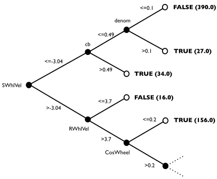
In order to demonstrate the application of the methodology, a specific symbolic pattern learning algorithm must be used for the generation of predicates. In this paper we use Decision Tree Induction for this purpose. Decision Tree Induction is a symbolic pattern learning algorithm that learns a disjunction of conjunctive rules describing a concept. A decision tree consists of two types of nodes; decision nodes and leaf nodes. A decision node contains an input attribute value. Each edge emanating from a decision node is labelled with one of the unique values in the domain of the attribute labelling the decision node. A leaf node is labelled using one of the classification labels. Each path of the tree from the root node to a leaf node is interpreted as a set of conjunctive expressions that lead to the classification label at the associated leaf node. The learning algorithm performs a greedy search of the space of all possible trees choosing decision node attributes that maximise the reduction in entropy of the class label. The C4.5 decision tree induction algorithm was used to learn the decision tree [34]. An example of the type of tree generated by the algorithm can be seen in Figure 2, where non-leaf nodes are labelled with variables, edges are labelled with potential variable states and leaf nodes are labelled with a failure classification. A predicate is derived by interpreting this structure as a conjunction of disjunctions.
Evaluation Method: To evaluate the effectiveness of the baseline predicate generated, 10-fold cross validation was
<=-3.04
>-3.04
<=0.49
>0.49
RWhlVel >3.7
FALSE (390.0)
TRUE (27.0)
FALSE (16.0)
TRUE (156.0)
<=0.1
>0.1
TRUE (34.0)
<=0.2
>0.2 SWhlVel
cb
denom
<=3.7
[image:10.612.338.553.72.250.2]CosWheel
Figure 2. Decision Tree Predicate Example
used to generate the confusion matrices for the adopted data mining algorithm. The data was partitioned into 10 stratified samples, then for each cross validation run, one of the partitions was used as the test sample, whilst the other nine were used as the training set.
Table III shows the evaluation of the predicates that were generated for all locations. The statistics shown in Table III relate to predicates generated using a baseline configuration of the Decision Tree Induction algorithm, i.e., no attempt was made to search for algorithm parameters which would yield the most effective predicates. In Table III the FPR
and TPR columns give the mean false positive and true positive rates taken across all 10 cross validations. A false positive here corresponds to the situation where a predicate incorrectly detects a state as being failure-inducing, whilst a true positive corresponds to a predicate correctly identifying a failure-inducing state. The AUC column shows the area under the ROC curve, as described in Section IV. TheComp
column gives the complexity of the derived predicates, where the stated value corresponds to the mean number of nodes in the decision tree for all 10 cross validations. TheVarcolumn gives the AUC variance across all 10 cross validations.
Table III
DECISION TREE INDUCTION RESULTS(NO SAMPLING)
Dataset FPR TPR AUC Comp Var 7Z-A1 2E-05 .9979 .9989 19.0 3E-08
7Z-A2 0 .9979 .9989 11.0 1E-08
7Z-A3 0 .9987 .9993 11.0 1E-08
7Z-B1 1E-04 .9435 .9717 58.1 3E-04
7Z-B2 0 .9691 .9845 5.0 1E-09
7Z-B3 0 .9654 .9827 9.0 9E-10
FG-A1 2E-04 .9906 .9951 100.3 7E-08 FG-A2 3E-03 .9807 .9891 136.4 3E-06 FG-A3 6E-04 .9878 .9936 75.9 3E-06 FG-B1 1E-04 .7929 .8964 61.1 1E-32 FG-B2 1E-05 .9584 .9791 172.3 1E-06 FG-B3 1E-04 .8223 .9111 62.8 6E-08 MG-A1 1E-09 .9938 .9969 7.0 1E-09 MG-A2 3E-04 .9938 .9967 7.2 7E-08
MG-A3 0 .9989 .9995 9.2 1E-32
MG-B1 0 .9740 .9870 7.0 1E-32
MG-B2 0 .9740 .9870 7.0 1E-32
MG-B3 0 .9728 .9864 3.2 1E-30
consistency with which effective predicates are generated.
D. Step 4: Model Refinement and Optimisation
Having generated and evaluated baseline predicates for error detection mechanisms, these models can now be refined by varying the parameters associated with the Decision Tree Induction algorithm. The results of this process are shown in Table IV. The columns of Table IV are the same as those given in Table III except for the S and N columns, which show the sampling level and the number of nearest neighbours used to generate the associated model respec-tively. Each entry in the S column also shows the type of sampling performed, where an O indicates oversampling and a U indicates undersampling. A total of 10 undersampling and 15 oversampling percentage levels were used in model refinement. These levels were distributed over the range [5,100] and [100,1500] for undersampling and oversampling respectively. The number of nearest neighbours considered were distributed over the range [1,15].
The entries in Table IV show that each of the models generated in the previous step were improved on, with respect to the mean AUC measure, during the predicate refinement process. In some cases this improvement is relatively small, occasionally less than a 0.000001 increase, but in the context of an error detection mechanism this increase can be significant. In almost all cases the variance of all models is increased, though it should be noted that these values remain extremely low.
In order to further validate the correctness of the results presented, a cross validation for each model had its predicate implemented as a runtime assertion in its corresponding code location, i.e., the location at which logging took place in order to generate the corresponding dataset. All fault injection experiments were then repeated to ensure that the
Table IV
DECISION TREE INDUCTION RESULTS(REFINED)
Dataset S N FPR TPR AUC Comp Var
7Z-A1 85(U) - 2E-05 .9982 .9991 19.0 2E-09 7Z-A2 300(O) 4 5E-05 .9983 .9991 34.3 5E-08
7Z-A3 500(O) 14 0 .9991 .9996 11.9 6E-32
7Z-B1 300(O) 12 1E-03 .9984 .9985 67.4 6E-07 7Z-B2 900(O) 6 3E-04 .9876 .9937 9.9 6E-05 7Z-B3 700(O) 7 7E-05 .9999 .9999 13.5 3E-08 FG-A1 500(O) 12 1E-03 .9966 .9977 113.7 8E-08 FG-A2 900(O) 1 4E-03 .9995 .9978 174.5 1E-08 FG-A3 500(O) 11 1E-03 .9963 .9974 113.2 1E-07
FG-B1 35(U) - 1E-02 .7963 .8964 68.3 2E-05
FG-B2 500(O) - 2E-04 .9628 .9813 173.1 3E-10 FG-B3 500(O) - 2E-04 .8229 .9114 61.2 3E-10
MG-A1 100(O) 2 0 .9938 .9969 7.0 1E-32
MG-A2 40(U) - 0 .9938 .9969 7.0 1E-32
MG-A3 5(U) - 0 .9989 .9995 9.0 1E-32
MG-B1 75(U) - 0 .9740 .9870 7.0 1E-32
MG-B2 5(U) - 0 .9740 .9870 7.0 4E-17
MG-B3 5(U) - 0 .9728 .9864 3.3 1E-28
observed FPR and TPR values were commensurate with the rates presented previously.
VIII. DISCUSSION
The results presented in Section VII demonstrate that the proposed methodology is capable of generating predicates for efficient error detection mechanisms. In particular, De-cision Tree Induction has, even under a basic configuration, been shown to be an effective and consistent method for generating predicates which exhibit a high true-positive rate and a low false-positive rate. Crucially, as the best derived predicate is represented as a decision tree, an example of which is shown in Figure 2, it can easily be extracted by in-terpreting the decision tree as a conjunction of disjunctions. This means that implementing an error detection mechanism based on a model generated using our methodology reduces to the, almost trivial, process of interpreting a decision tree. As fault injection analysis is commonly used in the validation of dependable software, the availability of fault injection data can often be assumed. This means that the main cost of applying the proposed methodology is associ-ated with data mining algorithms, which in-turn means that the cost of generating efficient predicates using our approach is related to dataset magnitude, the data mining algorithm being applied and the comprehensiveness of the refinement undertaken. In this paper, we have shown that using only a baseline configuration of a learning algorithm can yield highly efficient predicates and that even a naive parameter search can allow the efficiency of those predicates to be consistently improved.
program and whether that execution resulted in a failure. This focus contrasts with existing work on fault injection, which typically adopts the view that an error is any deviation from a fault-free execution, i.e, golden run. Interestingly, whilst the methodology proposed here is not directly appli-cable in this context, we believe that it is possible to adopt a similar approach in order to derive error detection predicates that can identify such deviations from a fault-free execution. The novelty of the proposed methodology is in the ap-plication of data mining to fault injection data in order to obtain predicates for efficient error detection mechanisms. The main advantage of this approach to predicate generation is that efficient error detection mechanisms can be obtained by design. This contrasts with current approaches, which often rely on the availability of a formal system specification or the experience of software engineers.
IX. CONCLUSION
A. Summary
In this paper, we presented a methodology for the genera-tion of predicates for efficient error detecgenera-tion mechanisms. The premise of the methodology is that, given a program location for which a detector component must be generated, optimised data mining techniques can be used to analyse fault injection data in order to generate efficient predicates for an efficient error detection mechanism. In contrast to current approaches, the methodology does not rely on a system specification or the experience of software engineers. In demonstrating the application of the methodology we have validated this premise, illustrating how data mining techniques can be used to generate predicates that exhibit high accuracy and completeness.
B. Future Work
In future work we plan to explore alternative approaches to the systematic design of predicates for error detection mechanisms. In particular, we will evaluate the applicability and impact of alternative data mining algorithms, fault models and system models in the generation of efficient error detection mechanisms.
REFERENCES
[1] J.-C. Laprie,Dependability: Basic Concepts and Terminology. Springer-Verlag, December 1992.
[2] A. Arora and S. S. Kulkarni, “Detectors and correctors: A theory of fault-tolerance components,” inProceedings of the 18th IEEE International Conference on Distributed Comput-ing Systems, May 1998, pp. 436–443.
[3] A. Jhumka, F. Freiling, C. Fetzer, and N. Suri, “An approach to synthesise safe systems,”International Journal of Security and Networks, vol. 1, no. 1, pp. 62–74, September 2006. [4] M. Hsueh, T. K. Tsai, and R. K. Iyer, “Fault injection
techniques and tools,” IEEE Computer, vol. 30, no. 4, pp. 75–82, April 1997.
[5] D. Powell, E. Martins, J. Arlat, and Y. Crouzet, “Estimators for fault tolerance coverage evaluation,” IEEE Transactions on Computers, vol. 44, no. 2, pp. 261–274, June 1995. [6] M. Hiller, “Executable assertions for detecting data errors
in embedded control systems,” in Proceedings of the 30th IEEE/IFIP International Conference on Dependable Systems and Networks, June 2000, pp. 24–33.
[7] J. Vinter, J. Aidemark, P. Folkesson, and J. Karlsson, “Re-ducing critical failures for control algorithms using executable assertions and best effort recovery,” inProceedings of the 37th IEEE/IFIP International Conference on Dependable Systems and Networks, July 2001, pp. 347–356.
[8] N. G. Leveson, S. S. Cha, J. C. Knight, and T. J. Shimeall, “The use of self checks and voting in software error detec-tion: An empirical study,” IEEE Transactions on Software Engineering, vol. 16, no. 4, pp. 432–443, April 1990. [9] A. Jhumka and M. Leeke, “Issues on the design of efficient
fail-safe fault tolerance,” in Proceedings International Sym-posium on Software Reliability Engineering, November 2009, pp. 155–164.
[10] S. S. Kulkarni and A. Arora, “Automating the addition of fault-tolerance,” in Proceedings of the 6th International Symposium on Formal Techniques in Real-Time and Fault-Tolerant Systems, September 2000, pp. 82–93.
[11] S. S. Kulkarni and A. Ebnenasir, “Complexity of adding failsafe fault-tolerance,” in Proceedings of the 22nd IEEE International Conference on Distributed Computing Systems, July 2002, pp. 337–344.
[12] M. Hiller, A. Jhumka, and N. Suri, “Propane: An environment for examining the propagation of errors in software,” in Pro-ceedings of the 11th ACM SIGSOFT International Symposium on Software Testing and Analysis, July 2002, pp. 81–85. [13] M. Hall, E. Frank, G. Holmes, B. Pfahringer, P. Reutemann,
and I. H. Witten, “The weka data mining software: An update,” SIGKDD Explorations, vol. 11, no. 1, pp. 10–18, June 2009.
[14] M. Hiller, A. Jhumka, and N. Suri, “An approach for analysing the propagation of data errors in software,” in
Proceedings of the 31st IEEE/IFIP International Conference on Dependable Systems and Networks, July 2001, pp. 161– 172.
[15] A. Jhumka, M. Hiller, and N. Suri, “An approach for de-signing and assessing detectors for dependable component-based systems,” inProceedings of the 8th IEEE International Symposium on High Assurance Systems Engineering, March 2004, pp. 69–78.
[17] C.-T. Lu, A. P. Boedihardjo, and P. Manalwar, “Exploiting efficient data mining techniques to enhance intrusion detec-tion systems,” inProceedings of the 2005 IEEE International Conference on Information Reuse and Integration, September 2005, pp. 512–517.
[18] S. J. Wenke Lee Stolfo and K. W. Mok, “A data mining frame-work for building intrusion detection models,” inProceedings of the 20th IEEE Symposium on Security and Privacy, May 1999, pp. 120–132.
[19] E. Clarke, O. Grumberg, and D. Peled,Model Checking. MIT Press, January 2000.
[20] D. A. Schmidt, “Data flow analysis is model checking of abstract interpretations,” in Proceedings of the 25th ACM SIGPLAN-SIGACT Symposium on Principles of Programming Languages, January 1998, pp. 38–48.
[21] P. Cousot and R. Cousot, “Abstract interpretation: A unified lattice model for static analysis of programs by construction or approximation of fixpoints,” in Proceedings 6th ACM SIGPLAN-SIGACT Symposium on Principles of Programming Languages, January 1977, pp. 238–252.
[22] M. D. Ernst, J. Cockrell, W. G. Griswold, and D. Notkin, “Dynamically discovering likely program invariants to sup-port program evolution,” IEEE Transactions on Software Engineering, vol. 27, no. 2, pp. 99–123, February 2001. [23] B. Demsky, M. D. Ernst, P. J. Guo, S. McCamant, J. H.
Perkins, and M. Rinard, “Inference and enforcement of data structure consistency specifications,” in Proceedings of the International Symposium on Software Testing and Analysis, May 2006, pp. 233–244.
[24] S. K. Sahoo, M. Li, P. Ramachandran, S. V. Adve, V. S. Adve, and Y. Zhou, “Using likely program invariants to detect hardware errors,” inProceedings of the 38th IEEE/IFIP Inter-national Conference on Dependable Systems and Networks, June 2008, pp. 70–79.
[25] D. Powell, “Failure model assumptions and assumption cov-erage,” inProceedings of the 22nd International Symposium on Fault-Tolerant Computing, July 1992, pp. 386–395. [26] M. Kubat, R. C. Holte, and S. Matwin, “Machine learning for
the detection of oil spills in satellite radar images,”Machine Learning, vol. 30, no. 2-3, pp. 195–215, 1998.
[27] T. Fawcett, “An introduction to roc analysis,”Pattern Recog-nition Letters, vol. 27, no. 8, pp. 861–874, June 2006. [28] N. Japkowicz, “The class imbalance problem: Significance
and strategies,” in Proceedings of the 2000 International Conference on Artificial Intelligence (ICAI, June 2000, pp. 111–117.
[29] L. Breiman, J. H. Friedman, R. A. Olshen, and C. J. Stone,
Classification and Regression Trees. Chapman and Hall/ CRC, January 1984.
[30] M. Pazzani, C. Merz, P. Murphy, K. Ali, T. Hume, and C. Brunk, “Reducing misclassification costs,” inProceedings of the 11th International Conference on Machine Learning, July 1994, pp. 217–225.
[31] K. M. Ting, “An instance-weighting method to induce cost-sensitive trees,” IEEE Transactions on Knowledge and Data Engineering, vol. 14, no. 3, pp. 659–665, May 2002. [32] P. Domingos, “A general method for making classifiers
cost-sensitive,” inProceedings of the 5th ACM SIGKDD Interna-tional Conference on Knowledge Discovery and Data Mining, July 1999, pp. 155–164.
[33] W. Fan, S. J. Stolfo, J. Zhang, and P. K. Chan, “Misclassi-fication cost-sensitive boosting,” in Proceedings of the 16th International Conference on Machine Learning, June 1999, pp. 97–105.
[34] J. Quinlan,C4.5: Programs for Machine Learning. Morgan Kaufmann, October 1992.
[35] M. Kubat and S. Matwin, “Addressing the curse of im-balanced training sets: One-sided selection,” inProceedings of the 14th International Conference on Machine Learning, January 1997, pp. 179–186.
[36] D. D. Lewis and J. Catlett, “Heterogeneous uncertainty sam-pling for supervised learning,” in Proceedings of the 11th International Conference on Machine Learning, June 1994, pp. 148–156.
[37] N. V. Chawla, K. W. Bowyer, L. O. Hall, and W. P. Kegelmeyer, “Smote: Synthetic minority over-sampling tech-nique,” Journal of Artificial Intelligence Research, vol. 16, no. 1, pp. 321–357, May 2002.
[38] B. Zadrozny, J. Langford, and N. Abe, “Cost-sensitive learn-ing by cost-proportionate example weightlearn-ing,” inProceedings of the 3rd IEEE International Conference on Data Mining, July, 2003, pp. 435–442.
[39] N. V. Chawla, D. A. Cieslak, L. O. Hall, and A. Joshi, “Auto-matically countering imbalance and its empirical relationship to cost,”Journal of Data Minining and Knowledge Discovery, vol. 17, no. 2, pp. 225–252, February 2008.
[40] 7-Zip, “http://www.7-zip.org/,” 2010.
[41] FlightGear, “http://www.flightgear.org/,” April 2009.