Recursive functional hardware descriptions using CλaSH

(1)

(2)

(3)

University of Twente

Master Thesis

Recursive Functional Hardware Descriptions

using C

λ

aSH

Author: Ingmar te Raa

Supervisors: Dr.Ir. J. Kuper Dr.Ir. J.F. Broenink Dr.Ir. C.P.R. Baaij Dr.Ir. R. Wester

Faculty of Electrical Engineering, Mathematics and Computer Science (EEMCS), Computer Architecture for Embedded Systems (CAES) group

(4)

(5)

Abstract

CλaSH is a functional hardware description language in which structural descriptions of combinational and synchronous sequential hardware can be expressed. The language is based on Haskell, from which it inherits abstraction mechanisms such as, the sup-port of polymorphism and higher-order functions. Recursion is another fundamental and commonly used abstraction mechanism in Haskell. In contrast with Haskell, the support of recursion in CλaSH is currently limited. This is considered a shortcoming by many CλaSH users.

Data-dependent recursive functions pose a problem for the current implementation of CλaSH. Currently, these recursive function definitions are unrolled by the compiler, in an attempt to produce finite circuits. In the case of data-dependent recursive functions, such finite circuit descriptions often cannot be found using unrolling, as it would require infeasibly large circuits, capable of handling all possible arguments.

(6)

(7)

Dankwoord

Allereerst wil ik de commissie bedanken voor het ondersteunen van mijn afstuderen. Jan, bedankt voor de uitvoerige gesprekken, waarbij ik volledig de aandacht kreeg. Graag bedank ik ook Christiaan voor zowel de waardevolle en uitvoerige feedback als inspiratie met be-trekking tot hardware ontwerp. Rinse, bedankt voor de goede begeleiding en gezelligheid op het kantoor.

Daarnaast wil ik de leden van de vakgroep CAES bedanken voor hun inspiratie en gezel-ligheid. Ik heb een goede indruk kunnen krijgen van zowel het leven van een promovendus, als de wetenschappelijke onderwijsvoering vanuit deze vakgroep. De gezelligheid tijdens de koffiepauzes en borrels die gepaard gingen met zowel goede discussies als droge humor: dit zorgde voor een werksfeer die nooit ging vervelen. In het bijzonder wil ik Arjan bedanken voor de hulp en inzichten die hij heeft gegeven met betrekking tot mijn afstuderen. En natu-urlijk mijn andere kantoorgenoot Guus. Samen met Rinse hebben wij heel wat lol gehad: essentieel voor de sfeer binnen het kantoor.

Ten slotte wil ik mijn vriendin Janneke bedanken, voor het onvoorwaardelijk steunen tijdens deze drukke periode.

Ingmar,

(8)

(9)

List of Figures

1.1 Trends in integrated circuits . . . 2

1.2 Applications domains of FPGAs in the industry, advertised by Altera Corpera-tion [3]. . . 2

2.1 Mealy machine circuit . . . 7

2.2 MAC circuit corresponding to the CλaSH description in Listing 2.1. . . 7

2.3 CλaSH compiler pipeline . . . 8

2.4 Lambda calculus. . . 9

2.5 Method of Sklyarov et al. . . 13

3.1 Expression grammar . . . 22

3.2 Type-system definitions . . . 23

3.3 Function definition syntax . . . 23

3.4 Naming rewrite rulesNJiK . . . 25

3.5 Sequentialize rewrite rulesSJeK. . . 27

3.6 Stack architecture . . . 29

3.7 Abstract representation of theCont . . . 30

3.8 Definition ofCall . . . 30

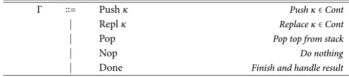
3.9 Stack instruction Γ definition . . . 30

3.10 Derive next rewrite rules . . . 32

3.11 Details of theContdatatype . . . 33

4.1 Implementation of stack architecture . . . 39

4.2 Detailed stack architecture . . . 40

(12)

(13)

List of Tables

3.1 Evaluation of Fibonacci next . . . 35

4.1 Appendix source code references . . . 38

5.1 Evaluation ofnextfunction in the case of Factorial . . . 44

5.2 Evaluation ofnextfunction in the case of Ackermann . . . 46

5.3 Results of the synthesis using Altera Quartus 15 tooling, targeting a Cyclone IV EP4CE22F17C6NFPGA. . . 47

5.4 Comparison of the synthesis results between results produced by the CλaSH compiler and [40] . . . 48 5.5 Comparison of the number of clock cycles before a algorithm finishes. The

(14)

(15)

1

Introduction

Computing devices are used to accomplish an ever increasing number of tasks. In the digital age we currently live in, these computer devices not only are omnipresent, the tasks they perform also evolve rapidly. The hardware that is used to accomplish these tasks, grows alongside with this trend. Due to innovations in fabrication techniques of transistors, used in for exampleCentral Processing Units (CPUs),Graphics Processing Units (GPUs), andField Programmable Gate Arrays (FPGAs), a larger number of these transistors can be packed into such chips.

To illustrate the trend that currently takes place in the evolution of computing devices, the number of transistors used in CPUs, GPUs, and FPGAs are shown in Figure 1.1. A period of 50 years show a rapid increase in transistor count. The largest transistor count displayed in Figure 1.1 contains more than twenty-billion transistors; an FPGA produced in 2014 by Xilinx [30]. To put that number in context, this is about 2.8 times the world population in 2014.

Figure 1.2 illustrates the wide variety of applications in which FPGAs are currently used. These applications vary from low demanding consumer applications to high demanding aerospace applications. In the early 90s the application domains of FPGAs were mainly net-working and telecommunication technologies. This indicates that: not only the capabilities of the FPGAs grow, but they are also deployed in a wider variety of application domains.

(16)

1970 1975 1980 1985 1990 1995 2000 2005 2010 2015 104

106 108 1010

Year of introduction

T

ra

n

si

st

o

r

co

un

t

[image:16.595.154.461.127.319.2]

FPGA GPU CPU

Figure 1.1 – Number of transistors in CPUs, GPUs, and FPGAs [4].

FPGA Automotive Broadcast Computer

& Storage Consumer

Embedded Vision

Industrial

Medical

Military / Aerospace / Government

Test & Measurement

Wireless

Wireline

[image:16.595.184.427.382.625.2]

(17)

1.1. PROBLEM STATEMENT AND APPROACH

Currently the most common HDLs that are used in the industry areVHSIC Hardware De-scription Language (VHDL)[1] andVerilog[2]. These languages have proven their power in the industry. It is however important to keep improving these languages, and exploring alternative languages compared to the existing ones.

In this thesis, the focus will lie on such an alternative: CλaSH [7]. CλaSH is a Functional HDL (FHDL) based on the semantics of the Haskell language in which structural descriptions of combinational and synchronous sequential hardware can be expressed. The language supports polymorphism and higher-order functions, properties inherited from the Haskell language.

1.1 Problem statement and approach

The ability to express recursive function definitions is fundamental in the Haskell language, and commonly used by developers using this language. In the CλaSH language, however, the ability to express recursive function definitions is limited. This is considered as a shortcoming by many CλaSH users [20, 26, 36, 37].

Research is conducted in this thesis to extend the support of recursion. As will be elaborated in this thesis, the ability to express recursion present in so-calleddata-dependentrecursive functions, is currently unsupported in CλaSH. The research question central to this thesis will therefore be:

» How can data-dependent recursive function definitions be supported by the CλaSH com-piler?

Several aspects related to this question need to be clarified, before this research question can be addressed. For instance, the exact limitations of CλaSH need to be identified. Furthermore, a type of hardware architecture need to be identified, capable of handling the recursive algorithms described in the CλaSH language. These structures must be derived automatically in order to be part of the CλaSH compiler.

1.2 Outline of this thesis

(18)

(19)

2

Background and Related Work

In this chapter, relevant background information and related work is elaborated. A basic understanding of the relevant topics discussed in this thesis, is established. Furthermore, relevant work is elaborated in form of a discussion. This provides the required knowledge which is needed to read the rest of this thesis.

Because CλaSH is central to this thesis, both the language and the compiler are elaborated. The reader should be able to understand how hardware is developed using the CλaSH lan-guage and the CλaSH compiler. The inner workings of the CλaSH compiler pipeline are also roughly discussed, without going into to much detail. Additionally, the current status of the support of recursion in CλaSH is elaborated.

Several different properties of recursive functions are distinguished in this research, which are also elaborated within this chapter. The properties of these recursive functions are ex-plained with the use of examples of such functions. Throughout the rest of this thesis, these properties are used to identify specific forms of recursion, for which these properties hold. Furthermore, the provided examples are used throughout this thesis to show the effects of the implementation of such recursive forms in reconfigurable hardware.

(20)

An overview of the CλaSH language and the CλaSH compiler, is provided in section §2.1. Background on recursion is elaborated in section §2.2: to enable the reader to distinguishes between various kinds of recursion. Then, in section §2.3, related work is evaluated. In this evaluation it will become clear that particular work is especially relevant to this thesis. Therefore a specific concept, used in the rest of this thesis, is further elaborated in section §2.4 to provide the necessary background to understand the rest of this thesis.

2.1 C

λ

aSH

CAES language for asynchronous hardware (CλaSH) [6, 7, 14] is a FHDL which borrows syn-tax and semantics from Haskell. The language allows a circuit designer to describe hardware using advanced Haskell language constructs like polymorphism and higher-order functions. Netlist of the circuits designed in CλaSH are produced by the compiler in commonly used HDLs like VHDL and Verilog. A circuit designer can use commonly available synthesis tooling, like Altera Quartus or Xilinx Vivado, to further synthesize the VHDL (or Verilog) produced by CλaSH, to a digital circuit. The CλaSH compiler also includes an interactive environment allowing a hardware developer to simulate the circuits developed in CλaSH, without the need of specifying a seperate test bench.

Throughout the past several years, CλaSH is used to describe circuits for applications in varying domains. This includes, domain specific processors: a Data-flow processor [27] and a Very Long Instruction Word (VLIW) processor [10]; the domain of computer algorithms: the n-queens algorithm [22] and the MUltiple SIgnal Classification (MUSIC) algorithm [21]; the domain of state space estimation using a particle filter [38], the domain of astronomy poly-phase filter bank [39], and an application in the domain of biology by means of an auditory model of a cochlea [11].

2.1.1 Hardware Design using CλaSH

In CλaSH, functions are used to describe hardware. A basic set of functions is provided in the CλaSH prelude library. This enables a circuit designer to design both combinational and synchronous sequential hardware. Types are used in CλaSH, to specify what kind of hardware needs to be compiled. One can for example use anUnsigned32 type to specify wires that can handle a 32 bit unsigned integer.

A special type, called aSignal, is used when a sequential synchronized circuits is described in CλaSH. ASignalcan be seen as aninfinitelist of samples, where each sample corresponds to a value at a specific moment in time. These moments are synchronized by a clock. Registers are used to capture the values of the samples. In other words, the state of theSignalis captured via registers. Combinational circuits are described, without the use of theSignal

(21)

2.1. CλASH

The CλaSH prelude library contains a classic machine model: the Mealy machine. Figure 2.1 shows this Mealy machine. Both the inputi and statesare input for the function f. The function f is the combinational function used to determine the outputoand the next state

s′. All the inputs and the output of f are of typeSignal. The next states′is captured in a register.

f

i o

[image:21.595.223.350.193.272.2]

s′ s

Figure 2.1 – Generic form of a Mealy machine as can be described by CλaSH

CλaSH hardware description example

To illustrate how CλaSH can be used to design circuits, an example is worked out in Listing 2.1 and Figure 2.2. Listing 2.1 shows a Mealy description of a Multiply ACcumulate (MAC) operation. The input of the Mealy description is a tuple(x,y)which contains the values

that need to be multiplied. The statesof the Mealy machine consist of an accumulator. The output of the MAC function is equal to the next states′.

Mathematically, one could express the result of the mac operation as:s′=s+x⋅y. Note the

similarities between the mathematical description and the hardware description in CλaSH. Figure 2.2 contains the resulting circuit corresponding to Listing 2.1.

mac s (x,y) = (s’,o) where

s’ = s + x * y o = s’

mac’ = mealy mac 0

Listing 2.1 – MAC hardware description defined in the CλaSH language.

+ ×

x

y o

s′ s

Figure 2.2 – MAC circuit corresponding to the CλaSH description in Listing 2.1.

2.1.2 Compiler pipeline

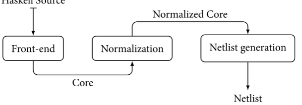
[image:21.595.320.468.484.557.2]

(22)

Haskell Source

Front-end Normalization Netlist generation

Netlist Core

[image:22.595.158.463.121.227.2]

Normalized Core

Figure 2.3 – CλaSH compiler pipeline

Front-end The CλaSH source code is presented to the front-end. This front-end processes the CλaSH source to anIntermediate Representation (IR)named Core. CλaSH uses the Glasgow Haskell Compiler (GHC) [35] for this step, which is an open source Haskell compiler. This Core IR is passed to the following step.

Normalization TheCoreproduced by the front-end is fed to the normalization step. This normalization step producesNormalised Core. In essence, the CλaSH compiler uses the normalisation step to make last step, the netlist generation, trivial.

Netlist Generation In the last step netlists are generated in the form of other, more low-level, HDLs. Currently the compiler supports the generation of VHDL, Verilog, and SystemVerilog netlists.

Intermediate representation

An IR namedCoreis used in the GHC and CλaSH compiler to ease the rewriting and analysis of the Haskell source. It is an abstract representation of the source in the form of a data structure. In GHC, a so-called ‘desugaring’ step produces the Core IR from the Haskell source. This abstract representation is based on SystemFC [34]: a polymorphic typedλ -calculus. Details of SystemFC are not described in this thesis as these details fall outside the scope of this thesis. In the CλaSH compiler, GHCs Core IR is rewritten to a subset of SystemFC in the Normalisation step.

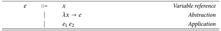
λ-calculus

(23)

2.1. CλASH

e ∶∶= x Variable reference

∣ λx→e Abstraction

[image:23.595.105.466.114.165.2]

∣ e₁e₂ Application

Figure 2.4 – Lambda calculus.

An untypedλ-calculus expression grammar is shown in Figure 2.4, as a basic example. It shows the construction of the three different basic syntax structures inλ-calculus; variables, abstractions and applications. Using this grammar, a computational step is described by a so-calledβ-reduction. This is a formal step where a substitution is performed:

(λx→e₁)e₂ Ô⇒ e₁[e₂/x]. (2.1)

In this computational step all occurrences ofxine1, are substituted bye2. Thisβ-reduction

can by applied to an example where a computational step is displayed:

(λx→x∗2)5 Ô⇒ 5∗2. (2.2)

Herexis substituted by 5 resulting in 5∗2.

In this thesis, a simply typedλ-calculus [23], is used as an basis for the abstract syntax. In such calculi, primitive data types such as characters, integers, or booleans are defined. In section §3.1, a detailed description of thisλ-calculus is provided.

2.1.3 Support for recursion in CλaSH

Currently recursion is supported by the CλaSH compiler to a certain degree. To determine to which extend support is currently available within the CλaSH compiler, two different kinds of supported recursion are distinguished;value recursionandrecursion via function definitions. The two are elaborated separately in the following subsections.

Value recursion

Currently CλaSH does supports value recursion in the form of feedback [5]. An example of such feedback is shown in Listing 2.2. In this example a counter circuit is described which uses a register to capture the state of aSignal s. ThisSignalcontains the value of the counter and is increased on each clock cycle.

counter = s where

s = register 0 (s + 1)

(24)

Recursion via function definitions

The support of recursion via function definitions is however limited: currently the CλaSH compiler uses unrolling in an attempt to synthesize recursive functions [6, pp. 127], which cannot always produce a result. The procedure creates a specialised function of the original recursive function that can be used for this unrolling. A fixed number of successive unroll actions is tried before the compiler quits the process. This limits the compiler in compile time and possibly the size of the generated netlists. If the base case is not found within the attempt of unrolling, an error is produced by the compiler.

Generally, if a function is data-dependent (see recursion properties defined in section §2.2.5) and the argument of the function is unknown at compile time, inlining of the function often doesnotproduce a desired result. The function must be able to handle all possible inputs of the function, which leads to an unfeasibly large hardware design, for even the simplest recursive functions. Thus, the support of generic data-dependent recursive descriptions is currently unsupported by the CλaSH compiler.

2.2 Recursion properties

Recursion is a central concept within this thesis. This section explains basic properties of recursion used in this thesis. This allows us to distinguish between several kinds of recursion. We focus on recursion via function definitions in the remaining parts of this thesis. From a mathematical point of view, a function is recursive if values in the function are calculated by using the same function: the function is defined in terms of itself. One may also speak of self referencing functions.

2.2.1 Linear, binary, and multiple recursion

Letnbe the number of recursive calls present in a function. Ifn=1 then one may speak of a

linear recursive function. The factorial function, as defined in equation (2.3), is an example of such a linear recursive function. Ifn=2 then the recursion function is called: a binary

recursive function. Finally, whenn>1, the function is called: a multiple recursive function.

The function that calculates the nth-Fibonacci’s number, as expressed in equation (2.4), is called a multiple — but more often called — binary recursive function.

f(n) = ⎧ ⎪ ⎪ ⎨ ⎪ ⎪ ⎩

1 ifn=1

n⋅f(n−1) ifn>1

, n∈_Z (2.3)

f(n) = ⎧ ⎪ ⎪ ⎨ ⎪ ⎪ ⎩

1 ifn=1, 2

f(n−1) + f(n−2) n>2

(25)

2.2. RECURSION PROPERTIES

2.2.2 Nested recursion

A recursive call can be nested, which occurs when the value of an argument of a recursive call is also calculated recursively. An example of such a nested recursive function is the Ackermann functionackeras defined in equation (2.5). Ifm,n>0 then a nested recursive

call is made.

acker(m,n) = ⎧ ⎪ ⎪ ⎪ ⎪ ⎨ ⎪ ⎪ ⎪ ⎪ ⎩

n+1 ifm=0

acker(m−1, 1) ifm>0 andn=0

acker(m−1,acker(m,n−1)) ifm,n>0

n,m∈_Z (2.5)

2.2.3 Tail recursion

A recursive function is tail recursive if a result of the function is directly determined by a recursive call. The factorial function described in (2.3) isnottail-recursive. However this function can be altered to become a tail recursive function. This is accomplished by means of an added argument that accumulatesm∗ntrough each iteration, as is shown in equation

(2.6).

f(m,n) = ⎧ ⎪ ⎪ ⎨ ⎪ ⎪ ⎩

n ifm=1

f(m−1,m∗n) ifm>1

, n,m∈_Z (2.6)

Developers often use this form of recursion, as compilers often can optimize this form of recursion. By means of a process called tail call elimination, tail recursive algorithms can sometimes be computed using only a fixed number of register’s, without the use of a growing call stack.

2.2.4 Indirect or mutual recursion

Recursive behaviour can also occur indirectly: if a recursive call is made via another function which is called by the function being defined, indirect recursion occurs. Indirect recursion via functions calling each other is often called mutual recursion. An example is when two functions f andgare specified and f usesgto calculate a value and vice versa.

2.2.5 Data-dependent recursion

(26)

2.3 Recursion in Reconfigurable Hardware

In this section, relevant research is covered to gather knowledge of how recursion is used in reconfigurable hardware. Relevant literature is consulted to accomplish this. First, the implementation approaches of recursive algorithms in reconfigurable hardware are covered. Secondly, other FHDLs similar to CλaSH will covered, while paying special attention to the support of recursion in these compilers.

The implementation approaches describing how to implement recursive algorithms in hard-ware descriptions are researched in §2.3.1. Although these approaches make use of existing low-level HDLs, they are of interest because of the produced hardware architectures. Their approaches to create hardware descriptions in these languages may reveal how recursive algorithms can be implemented in CλaSH.

Besides CλaSH, other compilers exists for FHDLs. These compilers are investigated, while paying extra attention to the support of recursion. In these compilers, the handling of re-cursion may be interesting. If the compiler strategies from other compilers are applicable to CλaSH, it is highly relevant for this thesis.

2.3.1 Approaches of implementing recursive algorithms in reconfigurable hardware

Several approaches for implementing recursion in reconfigurable hardware are compared in [31]. According to the author, all covered implementation approaches fall into two broad categories: either recursive calls are unrolled into a pipeline circuit, or, a stack architecture is used to implement the recursion.

In the survey [31] several characteristics are compared, such as: applicability, ease of use, occupied hardware resources, and stack usage. Regarding these characteristics, the most promising approach seems the one of Sklyarov et al. [24, 32, 33]. This approach is the only approach which can be applied to any recursive function, is easy to use, occupies a medium number of hardware resources, and requires a stack [31]. This approach is covered in the next section.

Sklyarov et al.

Sklyarov et al. propose a method for implementing recursive algorithms in hardware using Hi-erarchical Finite-State Machines (HFSMs)[24, 32, 33]. Recursive functions are implemented using a call stack, similarly as used in software, but parallelization occurs between recursive calls. Each function, recursive or not, is referred to as a single module. The combination of multiple modules represent the full circuit.

(27)

2.3. RECURSION IN RECONFIGURABLE HARDWARE

aspect of this approach comes from the invocation order of different modules, which is maintained by the use of a stack.

Figure 2.5 shows a general outline of the hardware architecture used by Sklyarov et al. The two stacks are controlled by the combinational circuit that updates the stacks depending on the current module and current state. The stacks can also be controlled externally via reset, push, and pop control signals.

combinational circuit

module stack FSM stack

input

output

control control

next module next state

[image:27.595.125.450.221.338.2]

current module current state

Figure 2.5 – Method of Sklyarov et al.

The method described by Sklyarov is useful for implementing recursive algorithms in VHDL. However, the methods are based on manually transforming Handel-C templates into VHDL, hence a language is used as reference which differs much compared to the functional ap-proach as used in CλaSH. Furthermore, the method requires manual implementation steps. Because the focus in this research is to extend the CλaSH compiler with the support of date-dependent recursive functions, we are more interested in automatic transformations instead of manual ones. The featured HFSM architectures however are of interest for this research, as these architecture can be used as templates for transformed algorithms.

2.3.2 Recursion in Functional Hardware Description Languages

Several research projects similar to CλaSH also generate circuits from functional hardware descriptions. However, the support of recursion varies in each project. A comparison of this related work is made in this section.

Edwards et al.

(28)

In their work, a series of rewrite steps is used to force the IR in a specific form called Continu-ation Passing Style (CPS) (explained in further detail in §2.4). This form of the IR allows the recursive algorithms to be handled in a stack architecture that is produced by the compiler.

Although the intention is clear in the papers, no formal rewrite rules are provided. The presented work provides sketches of the algorithms used to derive the stack architectures. Furthermore no details of the actual hardware architecture are provided. This makes it difficult to asses to which extend the research is conducted.

SAFL — Mycroft et al.

Statically Allocated parallel Functional Language (SAFL)[25] is a HDL in which each function is instantiated as a circuit at most once. The termstatically allocatedrefers to this property. As a result of this property, the size of circuits solely depends on the size of the text. Only primitive functions and operations are allowed to be duplicated. All other functions are instantiated once and calls to these functions will occur via multiplexers and arbiters.

Feedback is modeled as recursion in SAFL. Only tail-recursive function calls are possible in this model, because only those are statically allocatable, i.e., they require no stack. Listing 2.3 contains an example, copied from [25], which shows such feedback. A shift-add multiplier is implemented using tail recursion.

fun mult(x, y, acc) = if (x=0 | y=0) then acc

else mult(x<<1, y>>1, if y.bit 0 then acc+x else acc)

Listing 2.3 – shift add multiplier

If a circuit designer wants to compose the same circuit in parallel, the designer must dupli-cate the functions that describe the circuit. An example of this is shown in Listing 2.4 and Listing 2.5. In Listing 2.4, the function f is called twice in sequential order. The calls to this function are serialised and are handled mutually exclusively. This means that only one instance of the hardware is instantiated per function. One can use functions in parallel by du-plicating the function definitions of the same function. In Listing 2.5 multiple instantiations of the same function f are created to obtain such parallelism.

fun f x = ...

fun main(x,y) = g(f(x),f(y))

Listing 2.4 – f serial execution

fun f x = ... fun f’ x = ...

fun main(x,y) = g(f(x),f’(y))

(29)

2.3. RECURSION IN RECONFIGURABLE HARDWARE

Because SAFL allows only for tail recursive linear recursion, its handling of recursion does not advance the current situation of CλaSH. Furthermore, the single assignment form of SAFL poses an alternative view of the relation between code and hardware. It differs with the view CλaSH has with respect to the formation of hardware.

Verity — Ghica et al.

Ghica et al. describes the synthesis scheme behind Verity in a series of papers called Geom-etry of Synthesis [15–18]. It is a language which supports higher-order functions, mutable references, and uses an affine type system. In affine type systems, values may not be dupli-cated. In Verity this only holds for parallel and nested contexts, whereas duplication may occur in sequential context.

Recursion in Verity is supported only with the use of a fixed-point combinator. A fixed point combinatorfixis a higher-order function that satisfies:fix f = f (fix f). The name

is derived from the fixed-point equation: x = f x because, whenx = fix f, the fix point

combinator satisfies the fix point equation. An example of the usage of thisfixoperator is depicted in Listing 2.6. It illustrates how the (recursive) factorial function is implemented in Verity. Currently, the fix point operator is only unrolled in time by the Verity compiler. However, unrolling in space is theoretically explained in [18].

let fact = fix \f.\n. if n == 0$32 then 1$32 else n * f (n-1)

Listing 2.6 – Factorial in Verity, in this example 0$32 and 1$32 means a static 0 and 1 in a 32 bits integer.

Explicit constructs are used in Verity in order to indicate parallel or sequential operating hardware. A particular set of primitive types, called commands, are only allowed to be composed in parallel. For example, logical operations are not allowed to be composed in parallel, whereas for example memory assignment can be composed in parallel. Parallel constructs may not be used in fix-point combinators in Verity.

Recursion is treated as a special case in Verity. It requires the circuit designer to use spe-cific construct to use recursion. Furthermore the explicit constructs for creating parallel and sequential circuits differs much from CλaSH, as CλaSH handles every description com-binational by default and allow for sequential circuits trough the use of specific data-type constructions.

Lava — Bjesse et al.

(30)

in a standard Haskell environment. The program produces circuits by means of standard execution of the program.

Internally all circuits in Lava eventually are described by a tree-like data-structure. These data-structures can however describe an infinite tree, for example in the case of loops. There-fore, the synthesis function converts these infinite data-structures to a graph representation. Infinite cycles can be detected with the use of observable sharing [19] to obtain these graph representations.

Since finite recursion can be executed by the Haskell compiler, recursive circuits are also produced in Lava. However, the Lava compiler does not support recursion forms that depend on values that are unknown at compile time.

An example of a counter implemented in Lava is listed in Listing 2.7. The function has two signals as argument one for incrementing the counter and the other for resetting it. A register acts as memory element in the circuit and is initially set to 0. Two multiplexer elements, created with amuxfunction, handle the input signals. If the restart signal is high a 0 is chosen, otherwise the register output is chosen. The other multiplexer handles the incrementation of the counter. If the increase signal is high, the value of the register is increased, otherwise not. The resulting value is fed back in the register completing the circuit.

The example contains value recursion for theloopandregvalues. Like CλaSH it can handle such recursion, which is handled by the GHC compiler.

counter restart inc = loop where reg = register 0 loop

reg’ = mux2 restart (0, reg) loop = mux2 inc (reg’ + 1, reg’)

Listing 2.7 – Counter in Lava

Lava is an embedded language and produces circuits by the execution of Haskell programs. This is different from the approach CλaSH uses, as it uses a custom compiler to produce circuits. Recursive descriptions are supported at the level of execution of the Haskell program. This also means true data-dependent recursion cannot be expressed in Lava as it would require to inline all possible outcomes of the circuits. Furthermore, branching must be explicitly constructed in Lava. Branching in CλaSH leads to branching in the circuits, and no explicit constructions are needed.

2.3.3 Conclusion

(31)

2.4. CONTINUATION PASSING STYLE

abilities in terms of support of recursion, as they do support the use of true data-dependent recursion. However, Verity is very different compared to the CλaSH language.

The work of Edwards et al. is very similar compared to the work of the CλaSH compiler. They also use an intermediate representation which is very similar to the one used in CλaSH. Their work enables data-dependent recursive descriptions to be used in reconfigurable hard-ware. Furthermore Edwards et al. also use Haskell as a source language as CλaSH also does. Therefore the method that is described by Edwards et al. is further researched as a basis for this thesis.

2.4 Continuation Passing Style

As previously mentioned in section §2.3.2, in the work of Edwards et al., a series of rewrite steps is performed on a IR to derive a special form, enabling them with the support of recur-sion. This special form is calledContinuation Passing Style (CPS). The use of continuations was first described by A. van Wijngaarden in 1964. Later, van Wijngaarden would formulate what now is known as the continuation passing style [28].

CPS is a style of programming where each function call is accompanied with a continuation. A continuation is a description of what to do when a result of a function is ready — sometimes referred as the control. Instead of returning the result of the function, the function returns by calling this continuation with the result as argument. When a program is in CPS, the

controlis madeexplicit. As will become clear in the proceeding chapters, thisexplicit control

property of the CPS, is used to derive a stack architecture for recursively defined functions.

Example: Factorial function in CPS

In Haskell, one can write a function in continuation passing style by adding an extra argument, for examplek. This argument contains a continuation in the form of a lambda expression. This can be illustrated by the following example in Listing 2.8. In this example the factorial functionfact, also shown in (2.3), is CPS transformed tofact_cps.

-- regular factorial fact 0 = 1

fact n = n * (fact (n-1)) -- cps factorial

fact’ n = fact_cps n id fact_cps 0 k = k 1

fact_cps n k = fact_cps (n-1) (\r->k (n*r))

(32)

In the case ofn=0 the function returns by applying the continuationkto the result 1. When

n>0 a recursive call is made tofact_cpsapplied ton−1 and the continuation in the form

of the lambda expressionλ r → k(n∗r). The continuation describes what to do when

the result of the recursive call is available. In the case of the factorial function one should multiply the result withn. This is exactly what the lambda expression does: the lambda expression is applied to an argumentrwhich contains the result of the recursive call. This resultr is multiplied withnjust as in the originalfactdescription. A wrapper function,

fact’, applies the CPS transformed function tonvariable and to the identity function. Listing 2.9 evaluates the example withn=3. Continuations are nesting until the recursion

ends whenn = 0. The continuation is then applied to 1. After successively applying the

continuation to the intermediate results a final result of 6 is obtained.

-- cps factorial fact’ 3 = fact_cps 3 id

= fact_cps 2 (\r1->id (3*r1))

= fact_cps 1 (\r2->(\r1->id (3*r1)) (2*r2))

= fact_cps 0 (\r3->(\r2->(\r1->id (3*r1)) (2*r2)) ((1*r3))) = (\r3->(\r2->(\r1->id (3*r1)) (2*r2)) ((1*r3))) 1

= (\r2->(\r1->id (3*r1)) (2*r2)) (1*1) = (\r1->id (3*r1)) (2*1*1)

= id (3*2*1*1) = (3*2*1*1) = 6

Listing 2.9 – Haskell CPS example.

As can be seen in the listings, the original factorial function is transformed to a tail recursive function. However, while evolving this function, the added continuation argument increase and decrease in a stacked like manner. This CPS forms is not easily implemented in hardware. However, in the proceeding chapter, a formal methodology is presented derive a stack like architecture from a simply typed lambda calculus.

2.5 Conclusions

This chapter showed several topics of background information that is needed for the rest of this thesis. Two important conclusions can be distilled from the information provided in this chapter:

» A stack architecture can be used to implement data-dependent recursion in reconfig-urable hardware. Stack architectures are used in both manually derived implementa-tions of a data-dependent recursive algorithm (as described in §2.3.1), and automati-cally derived implementations of such algorithms (described in §2.3.2).

(33)

2.5. CONCLUSIONS

(34)

(35)

3

Methodology

In the previous chapter, both relevant literature and relevant topics as: CλaSH, terminology, and CPS are covered. In this chapter a methodology is developed that will elaborate on how to derive a stack architecture from data-dependent recursive functions.

To derive stack architectures from data-dependent function, a methodology is developed which splits the problem in several steps. First a basic abstract syntax is presented in order to represent recursive functions. This syntax is then used in rewrite rules to force the syntax into a specific form. These rewrite rules are based on the CPS transform, introduced in section §2.4. When the syntax is rewritten to this specific form, one can derive a stack architecture by a procedure also covered in this methodology.

The general outline of this chapter is as follows. In section §3.1, an abstract syntax is presented. This syntax is a basis for the rewrite rules introduced in section §3.2. These rewrite rules force a specific form of the syntax which makes it possible to generate a stack architecture as the one described in section §3.3. The generated stack architecture can then be fed to the CλaSH compiler, which can be used to produce netlist.

3.1 Abstract Syntax

(36)

3.1.1 Expression

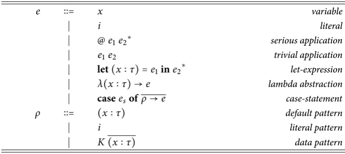
Figure 3.1 shows the expressions included in the abstract syntax. The expression grammar

e describes a basic typed lambda-calculus language extended with let expressions, case-statements, and a specific kind of application. Some expressions are not part of the allowed input syntax because these expressions play a specific role in the rewrite rules described in §3.2.

e ∶∶= x variable

∣ i literal

∣ @e₁e₂∗ serious application

∣ e₁e₂ trivial application

∣ let(x∶τ) =e₁ine₂∗ let-expression ∣ λ(x∶τ) →e lambda abstraction

∣ casee_sofρ→e case-statement

ρ ∶∶= (x∶τ) default pattern

∣ i literal pattern

[image:36.595.127.480.237.395.2]

∣ K(x∶τ) data pattern

Figure 3.1 – Expression grammare. Expressions marked with∗exists

only during the rewrite steps. They are not allowed as input grammar.

In the presented expression grammar, a distinction between different types of applications is made: applications can be eithertrivial or serious. This terminology is adopted from Reynolds [29]. Serious applications are marked with an extra @ sign before the application. This difference plays an important role in the rewrite steps discussed further in this chapter. Section §3.2.1 describes a rewrite step that marks the serious applications. In that section it will become clear how and why this notation is used. Serious applications are only present during the rewrite rules and are not allowed as input grammar.

In the case-expression, the scrutinee of the case-expression: es, is matched to the patterns

defined asρ. Three patterns are chosen to be included in the syntax. In the default pattern the scrutinee of the case-expression is simply bound to a variable. Another pattern is the comparison with a literal. If the scrutinee matches the literali, then the expression eis matched. Finally,escan also be matched to data constructors of algebraic data types. In this

caseKcontains the constructor identifier of the data type, and a list of binders(x∶τ)that

bind the variables of the data constructor. The notation(x∶τ)expands to(x₁ ∶ τ₁),(x₂ ∶

(37)

3.2. REWRITE RULES

3.1.2 Type system

The CλaSH compiler uses types to determine what kind of hardware should be generated. It is therefore important to incorporate types in the aforementioned abstract syntax. A basic type-system is used in the chosen abstract syntax. Figure 3.2 shows the definition of typeτ. A type atomwis used to identify different base types. For example Integers, Booleans, etcetera. A function operation on types:w→τ, is used to make function types. It is not possible to

describe higher-order function using this typing system. This simplifies the handling of the abstract syntax used in this thesis.

τ ∶∶= w atom

∣ w→τ function type

Figure 3.2 – Definition of typesτused in the abstract syntax.

3.1.3 Function definitions

Function definitions are included in the syntax as shown in Figure 3.3. Each function def-inition consist of an unique variable function namex. This function is bound to a type

warg→w_ret. The argument typew_argcan be used to declare multiple argument types and is

expanded with a function type as:warg→w_ret≡w₁→..→w_n →w_ret. The return typew_ret

contains the type of the return value.

FunDef ∶∶= x∶w_arg→w_ret=e Function definition

Figure 3.3 – Function definitionFunDef added to the abstract syntax.

This notation can be used to describe recursive functions. When the function name variable

x is used in the function expressionethen recursion occurs. This completes the abstract syntax used in the following sections for the rewrite rules.

3.2 Rewrite rules

It is now possible to describe rewrite rules using the abstract syntax constructed in the previous section. Sketches of the rewrite rules are provided in the paper of Edwards et al. [40]. However in order to formalize these steps, another paper from Danvy et al. [12] is used, that covers CPS transformation in great detail.

(38)

that describe what to do when a result of a recursive call is available. Rewrite rules covered in this section allow to obtain these continuations.

Fibonacci example

Throughout this section, a recursive function calculating the n-th Fibonacci number, as formulated in equation (2.4), has been chosen as example for the rewrite rules. Using the syntax defined in section §3.1 this function can be described as follows in (3.1). TheU32type

defines an unsigned 32-bits integer.

fib∶U₃₂→U₃₂=λn→casenof ⎧ ⎪ ⎪ ⎪ ⎪ ⎨ ⎪ ⎪ ⎪ ⎪ ⎩

1→1,

2→1,

n→ ((+) (fib(n−1))) (fib(n−2))

(3.1)

3.2.1 Marking serious applications

In the subsequent sections it will become clear that applications that are serious, effectively mark the places where the CPS transform should occur. In the first step we mark serious applications with the notation as defined in section §3.1. The transformation is only applied to the recursive calls, and therefore these are the places that needs to be marked.

Only those applications of which the recursive function that needs to be transformed and are fullysaturatedare marked. A function is saturated if the function is applied to all arguments of the function, or in other words the arity of the function is equal to the number of applied arguments. Using this terminology, only fully saturated recursive function applications are marked as serious applications. This procedure is illustrated by means of the Fibonacci example.

Fibonacci example

We now continue with the Fibonacci example initially described in section §3.2. In this function, x = fib; meaning the function name isfib. Fibonacci has only one argument,

therefore application is saturated whenfibis applied to that argument. Following this rule, equation (3.2) shows the result of marking all saturated recursive function applications. The serious markings @ are placed at each recursive call at the right place.

fib∶U₃₂→U₃₂=λn→casenof ⎧ ⎪ ⎪ ⎪ ⎪ ⎨ ⎪ ⎪ ⎪ ⎪ ⎩

1→1,

2→1,

n→ ((+) (@fib(n−1))) (@fib(n−2))

(39)

3.2. REWRITE RULES

3.2.2 Naming serious applications

Serious applications, introduced in the previous rewrite step, are provided with a name using thenaming-stepintroduced in this section. This step is executed to provide references to these expressions, which are used in the rewrite steps described later in this chapter.

The now following rewrite steps, follow a notation in the form of multiple rename rules

XJeK ↪ e

′_{. In this notation,}_X _{is the name of the rewrite step. Inside the double lined}

bracketsJ K, an input expressioneis placed. This expressioneis rewritten to the terme

′_,

if the expressionematches a described pattern. Note that expressione′can also contain rewrite termXJeKwhich need to be rewritten. The rewrite rules are applied recursively until

no further rewrite rules can be applied.

Figure 3.4 shows the rewrite rulesNJ Kthat form thenaming-step. This rewrite step is based

on the rewrite step described in the paper of Danvy et al. [12, p. 4].

NJxK ↪ x NJiK ↪ i

NJλ(x∶τ) →eK ↪ λ(x∶τ) →NJeK

NJ@e1e2K ↪ letx∶τ =NJe1KNJe2Kinx NJe1e2K ↪ NJe1KNJe2K

NJcaseesof ρ→eK ↪ caseNJesKofρ→NJeK

Figure 3.4 – Naming rewrite rulesNJiK

Serious applications @e1e2, that where introduced in §3.2.1, will be named in this rewrite

step. As can be seen, names are only introduced for these serious applications. The names are introduced in the form of a let-expression with an unique variablexbound to a type

τ. The type of the introduced variable is equal to the return type of the transformed func-tion, because only the recursive function calls are transformed. Again, notice that these let-expressions are only used in the rewrite steps and are not part of the allowed input syntax.

Fibonacci example

Workings of the naming-step are illustrated by applying these rules to the Fibonacci example. The rewrite rulesNJ Kare recursively applied to the result of the previous transformation

(where all serious applications are marked (3.2)). When this rewrite step is completed, all recursive function calls will be named in the form of let-expressions.

(40)

NJefibK↪NJ⋯n→ ((+) (@fib(n−1))) (@fib(n−2))K (3.3)

↪ ⋯n→ ((+)(let(x₁∶U₃₂) =fib(n−1)inx₁))

(let(x₂∶U₃₂) =fib(n−2)inx₂) (3.4)

As can be seen in the example, after applying the rewrite rule to the expression, each serious application is converted to a let-expression. In this case the unique names arex1 andx2.

The binders(x₁∶U₃₂), and(x₂∶U₃₂)bind these unique variables to the return type of the

functionwret, which is in this case equal to an integerU32.

3.2.3 Sequencing

In the rewrite step defined next, the previously defined let-expressions aresequenced. The presented rewrite rules are based on the ‘sequentialize’ rewrite rules defined in [12, p. 4]. These rewrite rules force the let-expressions to take a specific form. In this specific form, the following set of conditions is hold for all (sub-) expressions:

i let expressions do not occur in the bound expressione1of a let expression,

ii let expressions do not occur in applications,

iii the case scrutineeesdoes not contain let expressions.

Applying these conditions to the expressions yields asequenceof let-expressions, hence the namesequencing-step. A generic form of such a sequence is shown in (3.5).

⋯let(x₁∶τ₁) =e₁in let(x₂∶τ₂) =e₂in⋯let(x_n−₁∶τ_n−₁) =e_n−₁ine_n (3.5)

This sequence of let-expressions can be interpreted in terms of continuations in the CPS. Assume that the sequence of the let-expressions represent the execution order (from left to right) of each expression. If the first expressione1is executed and a result is returned returns,

expressione2can be executed, thereforee2is the continuation ofe1. Ife2then returns,e3

should be executed. This procedure repeats itself untilenis executed. By requiring previously

defined conditions to hold, the expressions take the form as shown in (3.5), hence a CPS is found.

Figure 3.5 contains the rewrite rules for thesequencing-stepSJ K. The bindings of

(41)

3.2. REWRITE RULES

SJxK ↪ (x, ∅) SJiK ↪ (i, ∅)

SJλ(x∶τ) →eK ↪ (λ(x∶τ) →letνine

′_,

∅)

where (e′, ν) =S_Je_K SJlet(x∶τ) =e1ine2K ↪ (e

′

2, ν1++ {(x∶τ) =e′₁} ++ν₂)

where (e′₁, ν₁) =S_Je_1K (e′₂, ν₂) =S_Je_2K SJe1e2K ↪ (e

′

1e′2, ν1++ν₂)

where (e′₁, ν₁) =S_Je_1K (e′₂, ν₂) =S_Je_2K SJcaseesof ρ→eK ↪ (casee

′

sofρ→letνine′, ν_s)

where (e′_s, ν_s) =S_Je_s_K (e′, ν) =S_Je_K S′JeK ↪ e

′

where (e′, ∅) =S JesK

Figure 3.5 – Sequentialize rewrite rulesSJeK.

A specific notation is used to indicate the introduction of these sequences:letνine′. Each collected binding out of the list{(x₁∶τ₁) =e₁},⋯,{(x_n∶τ_n) =e_n} ∈ν, is surrounded with

a let-expression, producing the desired let-sequence as in equation (3.5). Another notation is used to append two lists:++, which is common in Haskell.

In the case-statements, each pattern inρ→eintroduces its own let-sequence. Let expressions

are collected separately in a listν per pattern. The notationρ→letνine′denotes that a

let-sequence is introduced for each pattern.

All conditionsi⋯iiidefined earlier in this section are satisfied when applying the rewrite

rules in thesequence-stepSJ K. By construction, let-expressions only exist in the form of

(42)

Fibonacci example

The sequencing stepSJ Kcan now be applied to the output of the naming step calculated in

(3.4) in section §3.2.2. The results of applying these rules are shown in (3.6).

S′○N

JefibK↪SJ⋯n→ ((+)(let(x1∶U32) =fib(n−1)inx1)) (let(x₂∶U₃₂) =fib(n−2)inx₂)

K (3.6a)

↪ ⋯n→let(x₁∶U₃₂) = f ib(n−1)in

let(x₂∶U₃₂) = f ib(n−2)in((+)x₁)x₂ (3.6b)

The result of the sequencing step applied to the example can be interpreted as follows: first

fib(n−1)is bound to(x₁ ∶U₃₂)in the first let expression. The result of the function can

be accessed in the let expression viax1. Nextfib(n−2)is then bound to(x₂∶U₃₂)and the

result can be accessed via variablex2. Lastly, we sum bothx1andx2and this is the result of

the function.

In terms of continuations, firstfib(n−1)is executed. When the result offib(n−1)is known,

fib(n−2)can be executed. So the continuation of executingfib(n−1)isfib(n−2). When

the result offib(n−2)is known, one can sum both results and this is exactly the continuation

offib(n−2): namely((+)x₁)x₂.

3.3 Hardware Generation

Using the rewrite rules of previous section each recursive call is transformed into a sequence of let-expressions as shown in equation (3.5) in §3.2.3. In the same section, this sequence of let-expressions was interpreted in terms of CPS. In this section these let-sequences and this interpretation of these sequences are used to generate hardware.

Recall that in CPS each function call is accompanied with a continuation. This will also be the case in the generated hardware later described in this section. The continuations will consist of hardware descriptions which describe what to do when the result of the called function is available. However, when executing a function, another function call can occur accompanied with another continuation. In order to keep track of the continuations, a stack is introduced. This stack stores a continuation until the function returns the result.

Recall the sequence of let-expressions as defined in equation (3.5). Such a sequence is copied in equation (3.7), and annotated with Roman numerals.

let(x₁∶τ₁) =e₁in ´¹¹¹¹¹¹¹¹¹¹¹¹¹¹¹¹¹¹¹¹¹¹¹¹¹¹¹¹¹¹¹¹¹¹¹¹¹¹¹¹¹¹¹¹¹¹¹¹¹¸¹¹¹¹¹¹¹¹¹¹¹¹¹¹¹¹¹¹¹¹¹¹¹¹¹¹¹¹¹¹¹¹¹¹¹¹¹¹¹¹¹¹¹¹¹¹¹¹¹¶

(i)

let(x₂∶τ₂) =e₂in ´¹¹¹¹¹¹¹¹¹¹¹¹¹¹¹¹¹¹¹¹¹¹¹¹¹¹¹¹¹¹¹¹¹¹¹¹¹¹¹¹¹¹¹¹¹¹¹¹¹¹¹¸¹¹¹¹¹¹¹¹¹¹¹¹¹¹¹¹¹¹¹¹¹¹¹¹¹¹¹¹¹¹¹¹¹¹¹¹¹¹¹¹¹¹¹¹¹¹¹¹¹¹¹¹¶

(ii)

⋯ let(x_n−₁∶τ_n−₁) =e_n−₁in ´¹¹¹¹¹¹¹¹¹¹¹¹¹¹¹¹¹¹¹¹¹¹¹¹¹¹¹¹¹¹¹¹¹¹¹¹¹¹¹¹¹¹¹¹¹¹¹¹¹¹¹¹¹¹¹¹¹¹¹¹¹¹¹¹¹¹¹¹¹¹¹¹¹¸¹¹¹¹¹¹¹¹¹¹¹¹¹¹¹¹¹¹¹¹¹¹¹¹¹¹¹¹¹¹¹¹¹¹¹¹¹¹¹¹¹¹¹¹¹¹¹¹¹¹¹¹¹¹¹¹¹¹¹¹¹¹¹¹¹¹¹¹¹¹¹¹¹¶

(iii)

en

°

(iv)

(43)

3.3. HARDWARE GENERATION

Expression e1 is first executed, e2 needs to be executed aftere1 is finished, thus(ii) is a

continuation ofe1. This continuation(ii)belonging toe₂, is pushed on the stack, waiting

fore1to return. If the function returns, the continuation is removed from the stack and the

continuatione2is executed. However, the continuatione2can itself have a continuation, so

when executing e2, the continuation belonging toe3 is pushed on the stack. This process

repeats itself until the last continuationen is executed.

In the next subsection a stack architecture is introduced first. Then the results of previous sections are used in order to generate this stack architecture.

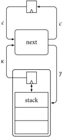
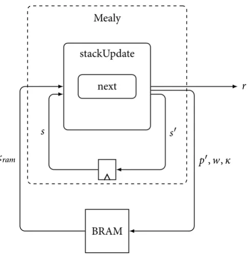
3.3.1 Stack Architecture

Figure 3.6 shows a generic version of the stack architecture used in this method. The stack ar-chitecture contains two registers which stores a callcand a continuationκ. The continuation register contains the top of the stack. Thenextfunction contains the logic to decide, given a call and a continuation, what to do next. This results in a stack instructionγfor updating the continuation stack and a follow up callc′

c _c′

[image:43.595.231.337.345.579.2]

γ κ

Figure 3.6 – Stack architecture

Continuations

(44)

τare also present in each continuationκ. Each continuation is present in the form of a data type constructor. Each continuationκis uniquely named.

Cont ∶∶= κ τ Continuations, context τ

Figure 3.7 – Abstract representation of theCont

Call

As mentioned in the intro of this section, a function can either be called or the function returns a result, when interpreted in CPS. A definition of these calls is introduced in Fig-ure 3.8. Types of the function call contains all the argument data types fetched fromτargin

the function definition of the recursive function (see §3.1.3) definition. Return calls contain the return type of the original function definitionwret.

Call ∶∶= F w_arg Function call arguments τ

∣ R w_ret Return call with return τ

Figure 3.8 – Definition ofCall

Stack Instructions

Another output of thenextfunction is a stack instructionγ∈Γ. This instruction is used to

update the continuation stack. Figure 3.9 describes Γ: the stack instructions.

Γ ∶∶= Pushκ Push κ∈Cont

∣ Replκ Replace κ∈Cont

∣ Pop Pop top from stack

∣ Nop Do nothing

[image:44.595.125.483.451.530.2]

∣ Done Finish and handle result

Figure 3.9 – Stack instruction Γ definition

ThePush instruction pushes a continuationκ on the stack while thePopinstruction re-moves the top instruction from the stack. Repl combines these two operations, resulting in a replacement of the top stack element. If nothing is to be done with the stack, theNop

instruction is used. Finally theDoneinstruction indicate the completion of a calculation.

3.3.2 Generating the Stack

(45)

Reconsider the general result of the sequencing step, as formulated in equation (3.5). After this step, the recursive function calls are in the form of a sequence of let-bindings. This sequence can be related to stack operations and data in the architecture.

Depending on the number of successive let-bindings in one sequence, different stack oper-ations are executed. Equation (3.8) shows the relation between the stack instructions and the let-sequences. The continuationsκ∈Contare denoted above the let-expressions. Notice

these continuations exactly relate to single let-expressions in a sequence. A tuple below the sequence denote what is to be fed to thenextfunction. The tuple consists of a callc ∈Call

and a stack operationγ∈Γ.

let(x₁∶τ₁) =e₁in ´¹¹¹¹¹¹¹¹¹¹¹¹¹¹¹¹¹¹¹¹¹¹¹¹¹¹¹¹¹¹¹¹¹¹¹¹¹¹¹¹¹¹¹¹¹¹¹¹¹¸¹¹¹¹¹¹¹¹¹¹¹¹¹¹¹¹¹¹¹¹¹¹¹¹¹¹¹¹¹¹¹¹¹¹¹¹¹¹¹¹¹¹¹¹¹¹¹¹¹¶

(c1,Push κ1)

κ1

³¹¹¹¹¹¹¹¹¹¹¹¹¹¹¹¹¹¹¹¹¹¹¹¹¹¹¹¹¹¹¹¹¹¹¹¹¹¹¹¹¹¹¹¹¹¹¹¹¹¹¹·¹¹¹¹¹¹¹¹¹¹¹¹¹¹¹¹¹¹¹¹¹¹¹¹¹¹¹¹¹¹¹¹¹¹¹¹¹¹¹¹¹¹¹¹¹¹¹¹¹¹¹¹µ

let(x₂∶τ₂) =e₂in ´¹¹¹¹¹¹¹¹¹¹¹¹¹¹¹¹¹¹¹¹¹¹¹¹¹¹¹¹¹¹¹¹¹¹¹¹¹¹¹¹¹¹¹¹¹¹¹¹¹¹¹¸¹¹¹¹¹¹¹¹¹¹¹¹¹¹¹¹¹¹¹¹¹¹¹¹¹¹¹¹¹¹¹¹¹¹¹¹¹¹¹¹¹¹¹¹¹¹¹¹¹¹¹¹¶

(c2,Repl(κ2))

⋯

κn−2

³¹¹¹¹¹¹¹¹¹¹¹¹¹¹¹¹¹¹¹¹¹¹¹¹¹¹¹¹¹¹¹¹¹¹¹¹¹¹¹¹¹¹¹¹¹¹¹¹¹¹¹¹¹¹¹¹¹¹¹¹¹¹¹¹¹¹¹¹¹¹¹¹¹·¹¹¹¹¹¹¹¹¹¹¹¹¹¹¹¹¹¹¹¹¹¹¹¹¹¹¹¹¹¹¹¹¹¹¹¹¹¹¹¹¹¹¹¹¹¹¹¹¹¹¹¹¹¹¹¹¹¹¹¹¹¹¹¹¹¹¹¹¹¹¹¹¹µ

let(x_n−₁∶τ_n−₁) =e_n−₁in ´¹¹¹¹¹¹¹¹¹¹¹¹¹¹¹¹¹¹¹¹¹¹¹¹¹¹¹¹¹¹¹¹¹¹¹¹¹¹¹¹¹¹¹¹¹¹¹¹¹¹¹¹¹¹¹¹¹¹¹¹¹¹¹¹¹¹¹¹¹¹¹¹¹¸¹¹¹¹¹¹¹¹¹¹¹¹¹¹¹¹¹¹¹¹¹¹¹¹¹¹¹¹¹¹¹¹¹¹¹¹¹¹¹¹¹¹¹¹¹¹¹¹¹¹¹¹¹¹¹¹¹¹¹¹¹¹¹¹¹¹¹¹¹¹¹¹¹¶

(cn−1,Repl(κn−1))

κn−1

«

en

±

(cn,Pop)

(3.8)

If the result ofe1is known,e2needs to be executed. This behaviour is produced by pushing

continuationκ1 on the stack. Ife2 returns, the top of the stack is replaced with e3. The

replacements are repeated for each continuation in the sequence until the last one. If the last continuation is executed, aNopinstruction is sent to the stack ending the continuations.

There are some cases where continuations can be omitted, which lead to a more efficient way of executing the transformed algorithm. Ifen=x_n−₁thenκ_n−₂is the last continuation of this

sequence, so a directNopinstruction can used andκn−1can be discarded as a continuation.

If a sequence contains only one let-expression, then no continuation need to be pushed on the stack so aNopstack instruction will suffice.

Deriving next function

Previous results now can be combined in deriving thenextfunction (as depicted in §3.3.1). Equation (3.9) contains a general outline of thenextfunction. The purpose of the final rewrite step introduced in this section, is to fill in the unknowns and generate thisnextfunction.

next(c,κ) =casecof ⎧ ⎪ ⎪ ⎨ ⎪ ⎪ ⎩

Fargs→e′

R r→caseκofα

(3.9)

The callccan be either afunction call Forreturn call R. The results of thenextfunction is in the form of a tuple containing a next callc′and a stack instructionγ. Continuations are han-dled when a return callRis invoked, in the form of a case-expression. This case-expression will use data patterns (see §3.1.1) for each continuation. The result of each continuation will also be a tuple with a next call and stack instruction. So elements ofαwill be in the form of

(46)

Figure 3.10 contains thederive nextrewrite rule_{DN R} ϕJ Kwhich collectse

′_and_α_{from an}

input expressione. This rewrite rule perform two tasks:

i All results ofnextthe function must be in the form of a tuple containing a call and stack instruction.

ii Continuations are collected in the form of a data pattern for a case-expression which handles the continuations.

This rewrite rule is called with a parameterϕto indicate if the continuation is the first in a sequence. This parameter is used in the helper functions_{DN R} ϕJ KandDN K ϕJ Kin

order to determine which stack operation belongs to the current expression. The parameter is initially true⊺. The result of the rewrite rule is a tuple(e′, α)which are used in thenext

function (3.9).

DN ϕJxK ↪ (DN R ϕJxK, ∅) DN ϕJiK ↪ (DN R ϕJxK, ∅) DN ϕJe1e2K ↪ (DN R ϕJe1e2K, ∅) DN ϕJlet(x1,τ) =e1inx2K ↪ (DN R ϕJe1K, ∅)

if x1=x₂

DN ϕJlet(x∶τ) =e1ine2K ↪ (DN K ϕJe1Kκ, κ→e

′

[x/r];α)

where (e′, α) =DN Je2K

κ=κ_newFV(let(x∶τ) =e₁ine₂) DN ϕJλb→eK ↪ (λb→e

′

, α)

where (e′, α) =DN ϕ JeK DN ϕJcaseesof ρ→eK ↪ (caseesof ρ→e′, α)

where (e′, α) =DN ϕ_Je_K

DN R ⊺

JeK ↪ (DN CJeK,Nop) DN R _Je_K ↪ (DN C_Je_K,Pop) DN K ⊺_Je_Kκ ↪ (DN C_Je_K,Push κ) DN K

JeKκ ↪ (DN CJeK,Repl κ) DN CJeK ↪

⎧ ⎪ ⎪ ⎨ ⎪ ⎪ ⎩

e[f/F] if f ∈FV(e)

R e otherw ise

Figure 3.10 – Derive next rewrite rulesDN ϕJ Kfor deriving next

(47)

The subroutines _{DN R} ϕJ Kand DN K ϕJ Kκ add stack instructions to the expressions.

These subroutines both use another subroutine _{DN C}J Kwhich makes a call instruction

of the currently handled expression. This is accomplished by checking if the original func-tion namef is in the free variables of the currently handled expressione. If this is true, the function name is simply substituted by the constructor nameF. Otherwise the expression must be a return statement, so a return constructor nameRis applied to the expressione.

Another task in deriving thenextfunction is the collection of continuations. As can be seen in the definition of the rewrite rules, continuations are only introduced for each let-expression where (x1≠x₂). As already stated, the continuations are in the form ofκ(x∶τ) →e_κ. The

data constructorκ is named uniquely and will be of the form as presented in Figure 3.11. The first continuation will only contain the free variables used in the rest of sequence of continuations. Because the intermediate results of each successive continuation also can be used in the rest of the continuations, this value is added to the data constructor of the continuation when the result of the continuation is known.

Cont ∶∶= κ₁τ_{f v} κ₁with free variables τ_{f v}

∣ κ₂τ_{f v}τ_x₁

∣ κ₃ τ_{f v}τ_x₁τ_x₂

Figure 3.11 – Details of theContdatatype

This completes thederive-nextrewrite step as both taskiandiiformulated earlier in this sec-tion are handled by this rewrite step. The remainder of this chapter will cover the applicasec-tion of thederive-nextrewrite step to the Fibonacci example.

Fibonacci example

Returning to the Fibonacci example, thenextdescription can be generated by applying the

(48)

collects the rewritten function descriptione′, and the continuationsα.

DN ⊺ ○S′○N_Je_fib_K↪DN ⊺_J⋯n→let(x₁∶U₃₂)) = f ib(n−1)

in let(x₂∶U₃₂) = f ib(n−2)in((+)x₁)x_2K (3.10a)

↪ (e′, α) (3.10b)

,where

e′=casenof ⎧ ⎪ ⎪ ⎪ ⎪ ⎨ ⎪ ⎪ ⎪ ⎪ ⎩

1→ (R1, Nop)

2→ (R1, Nop)

n→ (F(n−1), Push(κ₁n))

(3.10c) α= ⎧ ⎪ ⎪ ⎨ ⎪ ⎪ ⎩

κ1n→ (F(n−2),Repl(κ₂n r))

κ2n x1→ (R(x₁+r),Pop)

(3.10d)

These results can now be plugged into thenextdescription from (3.9). Equation (3.11) shows the resultingnextfunction for the Fibonacci example.

next(c,κ) =casecof ⎧ ⎪ ⎪ ⎪ ⎪ ⎪ ⎪ ⎪ ⎪ ⎪ ⎪ ⎪ ⎪ ⎪ ⎨ ⎪ ⎪ ⎪ ⎪ ⎪ ⎪ ⎪ ⎪ ⎪ ⎪ ⎪ ⎪ ⎪ ⎩

Fn→casenof ⎧ ⎪ ⎪ ⎪ ⎪ ⎨ ⎪ ⎪ ⎪ ⎪ ⎩

1→ (R1, Nop)

2→ (R1, Nop)

n→ (F(n−1), Push(κ₁n))

R r→caseκof ⎧ ⎪ ⎪ ⎪ ⎪ ⎨ ⎪ ⎪ ⎪ ⎪ ⎩

κ1n→ (F(n−2), Repl(κ₂n r))

κ2n x1→ (R(x₁+r), Pop)

κ0→ (R r,Done)

(3.11)

This provides anextdescription for the for the stack architecture described in §3.3.1. This

nextdescription, together with a basic description for the stack architecture, can be fed to the CλaSH compiler to generate hardware.

Table 3.1 contains an evaluation of thenextfunction, as defined in equation (3.11), with an input ofF3. Each successive application of thenextfunction is numbered in this table. Each row consist of anextfunction applied applied to a callcand continuationκ. The resulting tuple(c′,γ)is listed together with the stack after applying the stack instruction.

The result of the calculation of Fibonacci 3 is known after 6 successive applications of thenext

(49)

next(c,κ) = (c′,γ) Stack

[κ₀]

1 next(F3,κ₀) = (F2,Push(κ₁3)) [κ₁3,κ₀]

2 next(F2,κ₁3) = (R1,Nop) [κ₁3,κ₀]

3 next(R1,κ₁3) = (F1,Repl(κ₂3 1)) [κ₂3 1,κ₀]

4 next(F1,κ₂3 1) = (R1,Nop) [κ₂3 1,κ₀]

5 next(R1,κ₂3 1) = (R2,Pop) [κ₀]

6 next(R2,κ₀) = (R2,Done) [κ₀]

(50)

Recursive functional hardware descriptions using CλaSH

University of Twente

Master Thesis

Recursive Functional Hardware Descriptions

using C

λ

aSH

Contents

List of Figures

List of Tables

1

Introduction

1.1

Problem statement and approach

1.2

Outline of this thesis

2

Background and Related Work

2.1

C

λ

aSH

2.2

Recursion properties

2.3

Recursion in Reconfigurable Hardware

2.4

Continuation Passing Style

2.5

Conclusions

3

Methodology

3.1

Abstract Syntax

3.2

Rewrite rules

3.3

Hardware Generation