University of Warwick institutional repository: http://go.warwick.ac.uk/wrap A Thesis Submitted for the Degree of PhD at the University of Warwick
http://go.warwick.ac.uk/wrap/36270
This thesis is made available online and is protected by original copyright. Please scroll down to view the document itself.
Calibration of Interest Rate Term Structure and
Derivative Pricing Models
Kin Pang
Submitted for the degree of Doctor of Philosophy
Warwick University
Financial Options Research Centre, Warwick Business School
TABLE OF CONTENTS
CHAPTER 1. INTRODUCTION 1.1
1.1 BACKGROUND 1.1
1.2 OBJECTIVE 1.2
1.3 OVERVIEW 1.2
CHAPTER 2. MODELLING ISSUES AND TERM STRUCTURE
DERIVATIVE PRICING REVIEW 2.1
2.1 INTRODUCTION 2.1
2.2 MODELLING ISSUES 2.2
2.3 PRICING REVIEW 2.6
2.4 MODELLING REVIEW 2.8
2.4.1 Short Rate Models 2.9
2.4.1.1 One-factor No-Arbitrage Short Rate Models 2.10
2.4.1.2 Multifactor No-Arbitrage Short Rate Models 2.11
2.4.2 HJM Approach to Term Structure Modelling 2.11
2.5 PRICING METHODS 2.13
2.6 REFERENCE 2.16
CHAPTER 3. LITERATURE REVIEW ON CALIBRATION OF INTEREST
RATE TERM STRUCTURE MODELS TO OPTIONS PRICES 3.1
3.2 CALIBRATING SHORT RATE MODELS TO OPTIONS PRICES 3.2
3.2.1 Hull and White (1993a, 1995, 1996) 3.2
3.3 CALIBRATING HEATH, JARROW AND MORTON TYPE MODELS TO
OPTIONS PRICES 3.5
3.3.1 Amin and Morton (1994) 3.5
3.3.2 Brace and Musiela (1994) 3.8
3.3.3 Brace, Gatarek and Musiela (1995) 3.11
3.4 SUMMARY 3.13
3.5 REFERENCES 3.13
CHAPTER 4. CALIBRATION OF SHORT RATE MODELS 4.2
4.1 INTRODUCTION 4.2
4.2 CALIBRATION OF SHORT RATE MODELS 4.3
4.2.1 Arrow-Debreu Pure Security Prices, Kolmogorov Forward and
Backward Equations 4.4
4.2.2 BDT tree construction 4.7
4.2.2.1 Fitting Black, Derman and Toy to the Interest Rate Term
Structure Only 4.7
4.2.2.2 Fitting Black, Derman and Toy to both the Interest Rate and
Volatility Term Structures 4.9
4.2.3 HW tree construction 4.11
4.2.3.1 Fitting Hull and White tree to Interest Rate Term Structure Only _4.12 4.2.3.2 Fitting Hull and W tree to Interest Rate and Volatility Term
4.3 CALIBRATION TO OPTIONS PRICES 4.16 4.3.1 Fitting to the Interest Rate Term Structure and Options Prices _ 4.17
4.3.1.1 Example 1: Calibration to Caplets Prices 4.20
4.3.1.2 Example 2: Calibration to Floorlet Prices 4.22
4.3.2 Misspecification Issues 4.24
4.4 MULTIFACTOR SHORT RATE MODELS 4.29
4.5 SUMMARY 4.31
4.6 REFERENCES 4.32
CHAPTER 5. DUFFIE AND KAN AFFINE MODELS OF THE TERM
STRUCTURE OF INTEREST RATES 5.2
5.1 INTRODUCTION 5.2
5.2 THE DUFFIE AND KAN AFFINE MODELS AND THE GENERALISED
COX INGERSOLL AND ROSS INTEREST RATE MODEL 5.6
5.2.1 Duffle and Kan Affine Model 5.7
5.2.2 The Duffle and Kan Affine Yield Model 5.9
5.2.3 Duffle and Kan Non-Negative Affine Yield Model 5.10
5.2.4 Converting a Duffle and Kan Affine Model to a Yield Model 5.11 5.2.5 The Generalised Cox, Ingersoll and Ross Interest Rate Model 5.13
5.3 IMPLEMENTATION AND CALIBRATION ISSUES 5.14
5.3.1 The Indirect Approach 5.15
5.3.2 The Direct Approach 5.18
5.4 EQUIVALENCE BETWEEN GENERALIZED CIR INTEREST RATE AND
5.4.1 Degrees of Freedom 5.22
5.4.2 Equivalence 5.24
5.5 SUMMARY 5.25
5.6 APPENDIX 5.25
5.7 REFERENCES 5.27
CHAPTER 6. IMPLEMENTING THE HEATH JARROW AND MORTON
APPROACH TO TERM STRUCTURE MODELLING 6.2
6.1 INTRODUCTION 6.2
6.2 HEATH, JARROW AND MORTON FORWARD RATE TREES 6.3
6.3 MONTE CARLO SIMULATIONS 6.9
6.3.1 Simple Monte Carlo Simulations 6.9
6.3.2 Efficient Monte Carlo Simulations 6.10
6.3.2.1 Martingale Variance Reduction 6.12
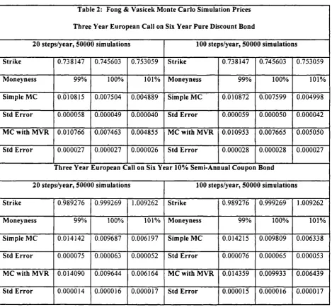
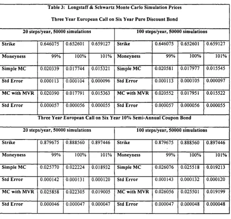
6.3.2.2 Stochastic Volatility Example 1: Fong and Vasicek (1991) 6.15 6.3.2.3 Stochastic Volatility Example 2: Longstaff and Schwartz (1992) 6.17
6.4 HJM SIMPLIFICATIONS 6.19
6.4.1 Gaussian Heath, Jarrow and Morton and Numerical Integration 6.19
6.4.2 Markovian Heath, Jarrow and Morton 6.21
6.5 SUMMARY 6.23
6.6 REFERENCES 6.24
7.1 INTRODUCTION 7.2
7.1.1 Review of Conventional Approaches 7.3
7.1.1.1 Principal Components Analysis Calibration 7.3
7.1.1.2 Implied Volatility Factors 7.5
7.2 REVIEW OF THE KENNEDY GAUSSIAN RANDOM FIELD TERM
STRUCTURE MODEL 7.7
7.2.1 Example 1: Hull-White Model 7.9
7.2.2 Example 2: Gaussian Heath, Jarrow and Morton 7.10
7.3 COVARIANCE FUNCTION, CONTINUITY AND SMOOTHNESS 7.11
7.4 IMPLIED COVARIANCE OF ZERO COUPON YIELD CHANGES AND
HJM CALIBRATION 7.16
7.5 THE PRICING OF CONTINGENT CLAIMS 7.18
7.5.1 Pricing of Caps 7.21
7.5.2 Pricing of European Swaptions 7.22
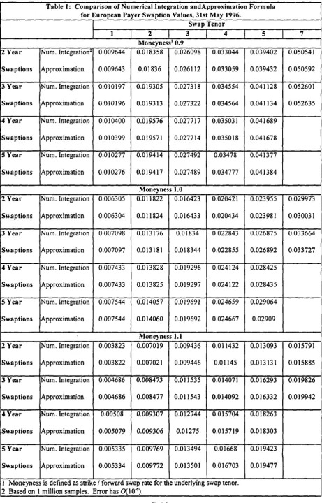
7.5.3 An Approximate European Swaption Pricing Formula 7.25
7.6 DATA 7.29
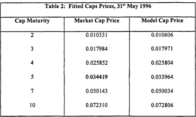
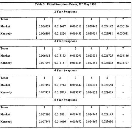
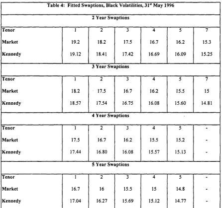
7.7 CALIBRATION TO CAPS AND SWAPTIONS PRICES 7.29
7.8 SUMMARY 7.33
7.9 APPENDIX 7.33
7.10 REFERENCES 7.38
8.1 INTRODUCTION 8.1
8.2 RESULTS FROM MUSIELA AND RUTKOWSKI (1996) 8.3
8.3 PRICING OF RESETTABLE CAPLET 8.8
8.4 PRICING OF RESETTABLE FLOOR 8.13
8.5 NUMERICAL RESULTS 8.14
8.5.1 Monte Carlo Simulations 8.15
8.6 APPROXIMATIONS 8.16
8.7 CALIBRATION ISSUES 8.21
8.8 SUMMARY 8.23
8.9 APPENDIX 8.24
8.10 REFERENCES 8.24
CHAPTER 9. SUMMARY AND FURTHER RESEARCH 9.1
9.1 SUMMARY 9.1
9.2 FURTHER RESEARCH 9.4
GLOSSARY OF TERMS 10.1
NOTATIONS 11.1
ACKNOWLEDGEMENTS
I am extremely grateful to Stewart Hodges for his constant support, encouragement and advice throughout my work towards this thesis. I would not have been able to produce this thesis without his guidance.
I wish to thank the staff at the Financial Options Research Centre, Warwick Business School. In particular, I would like to express my
gratitude to Les Clewlow and Chris Strickland for showing me the ropes. I thank Gail Dean and Asha Leer for their secretarial assistance.
I wish to thank Andrew Carverhill at Hong Kong University of Science and Technology for many fruitful discussions. I thank Nick Webber at Warwick University for introducing me to financial derivatives during my study for my Masters degree at Warwick University.
ABSTRACT
We argue interest rate derivative pricing models are misspecified so that when they are fitted to historical data they do not produce prices consistently with the market. Interest rate models have to be calibrated to prices to ensure consistency. There are few published works on calibration to derivatives prices and we make this the focus of our thesis.
We show how short rate models can be calibrated to derivatives prices accurately with a second time dependent parameter. We analyse the misspecification of the fitted models and their implications for other models.
We examine the Duffle and Kan Affine Yield Model, a class of short rate models, that appears to allow easier calibration. We show that, in fact, a direct calibration of Duffle and Kan Affine Yield Models is exceedingly difficult. We show the non-negative subclass is equivalent to generalised Cox, Ingersoll and Ross models that facilitate an indirect calibration of non-negative Duffle and Kan Affine Yield Models.
We examine calibration of Heath, Jarrow and Morton models. We show, using some experiments, Heath, Jarrow and Morton models cannot be calibrated quickly to be of practical use unless we restrict to special subclasses. We introduce the Martingale Variance Technique for improving the accuracy of Monte Carlo simulations.
We examine calibration of Gaussian Heath Jarrow and Morton models. We provide a new non-parametric calibration using the Gaussian Random Field Model of Kennedy as an intermediate step. We derive new approximate swaption pricing formulae for the calibration.
We examine how to price resettable caps and floors with the market-Libor model. We derive a new relationship between resettable caplets and floorlets prices. We provide accurate approximations for the prices. We provide practical approximations to price resettable caplets and floorlets
1. INTRODUCTION
1.1 BACKGROUND
The investments banks of the 1990's offer to their customers many sophisticated products that were not available in earlier times. Many of these products are financial derivatives, also called options and contingent claims, whose values are derived from the value of fundamental financial variables such as a stock index level or an interest rate. Financial derivatives can be used for many purposes including hedging against adverse movements of specified financial variables and providing an efficient means to express opinions on the movements of financial variables that cannot be so easily achieved without the use of financial derivatives. The importance of financial derivatives to the banking sector is
illustrated by their diversity and trading volume. Any bank that can offer these products, and know how to price and hedge their exposures accurately, will have a competitive advantage.
Ever since Black and Scholes (1973) and Merton (1973) laid down the fundamental principles for the pricing of options, banks have been offering increasingly complicated financial derivatives and have been using increasingly sophisticated methods to price financial derivatives. However, despite rapid advancement in our knowledge and ability to model options prices, we will never be able to replicate the real world with all its fine details precisely. Thus options pricing models have to be calibrated to compensate for their deficiencies and to ensure that they comply with market data. We use the term calibration for the process of choosing the parameters that allow the model to agree with market data.
following chapters we shall focus on the issue of calibration. We restrict our attention to interest rate derivative pricing models although the problems we highlight will apply equally to other areas such as equity and commodity options pricing.
1.2 OBJECTIVE
Banks have been calibrating their options pricing models to market prices and historical data ever since they started applying options pricing models. However, there is little academic work on these issues and the published work is scarce. We wish to contribute to the literature in this area by examining the issues involved, surveying how the different interest rate pricing models can be calibrated and providing suggestions of our own.
1.3 OVERVIEW
The thesis begins in Chapter 2 by defining the general mathematical
framework and discussing the modelling issues one has to consider when devising a suitable interest rate derivative pricing model. We distinguish between the two major branches of models, the equilibrium and evolutionary models, and explain why we and practitioners prefer to work with the latter. We also provide a review of the pricing methodology and a review of the various interest rate term structure and derivative pricing models. Finally we review some numerical pricing methods. Chapter 3 provides a review and analysis of some previous calibration work published in the academic literature.
Chapter 4 examines the short rate models and their calibration. The short rate models are perhaps the simplest of the interest rate models of the term
efficient numerical methods and provide analytical tractability. In chapter 4 shows how short rate models can be calibrated easily and highlights some problems inherent to short rate models that may deter their use. We also use short rate models as a basis for analysing model misspecification and its consequences for pricing and hedging.
Chapter 5 examines a model that may have been designed to aid calibration and overcome some of the problems presented by the short rate models. The affine yield model of Duffle and Kan (1996) determines the evolution of an entire interest rate term structure from the joint evolution of a number of reference zero coupon yields. This is certainly attractive, since not only zero coupon yields and their volatilities are relatively easy to ascertain, but also because interest rate derivatives have payoffs defined with reference to only a small number of zero coupon yields. In chapter 5 we show the Duffle and Kan model is unlikely to be used much in practice because it is exceedingly difficult to specify parameters for the model such that the state variables are consistent with being zero coupon yields and even more difficult to calibrate to a volatility term structure or options
prices. Furthermore, we illustrate that non-negative Duffle and Kan yield models are in fact equivalent to a class of short rate models we call Generalised Cox, Ingersoll and Ross models that are far easier to calibrate. Anyone wishing to work with a non-negative Duffle and Kan Yield model should start with a Generalised Cox, Ingersoll and Ross model instead.
We will have seen in Chapters 4 and 5 that a major problem with the models considered there is ensuring that the models produce realistic volatility factors for the zero coupon yields. Chapter 6 considers the general approach of Heath, Jarrow and Morton (1992) that models interest rates more realistically than the
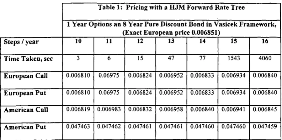
inappropriate, at least in its full generality, because of its intensive computational requirements. Chapter 6 provides timings to show how calibration would be too slow for practical needs even when tricks are used to speed up computation. Chapter 6 reproduces much of Carverhill and Pang (1995). Chapter 6 concludes with a review of some of the subclasses of Heath Jarrow and Morton models that may permit easier calibration, illustrating the compromise between tractability and realism one usually encounters in modelling.
Chapter 7 examines the calibration of Gaussian Heath, Jarrow and Morton models: the class in which interest rates are normally distributed. Although negative interest rates are possible and undesirable, some interest rate derivatives are not affected significantly by the possibility that negative interest rates may occur. A Gaussian Heath Jarrow and Morton model may be acceptable for this situation and these models are relatively easy to calibrate. However, common approaches have not been very satisfactory and in Chapter 7 we propose a new method that we believe is superior. We argue that it may be preferable to calibrate Gaussian Heath Jarrow and Morton models using the Gaussian Random Field Model of Kennedy (1994) as an intermediate step.
market-Libor model can be calibrated for the other approximation when higher accuracy is needed.
2. MODELLING ISSUES AND TERM STRUCTURE DERIVATIVE
PRICING REVIEW
2.1 INTRODUCTION
In this chapter we review the concept of modelling to explain what models aim to achieve in the context of interest rate term structure modelling and
derivative pricing. We provide a review of the contingent claims pricing
methodology in modern finance and a review of the different classes of interest rate models published in the academic literature. For calibration to be achieved easily, the models must offer either analytical prices or efficient numerical pricing
algorithms for common options. It is important to understand when efficient numerical methods would be available so we also review general pricing methods.
2.2 MODELLING ISSUES
It is possible to consider the pricing of securities within a model of the economy, such as in the equilibrium model of Cox, Ingersoll and Ross (1985a, 1985b), and to deduce prices endogenously as a function of the assumed investor and economic properties. However, such models are unlikely to remain tractable if they are to capture fine details of the real world and to date equilibrium models have provided few solutions to practical problems. Furthermore, the equilibrium models fail to reproduce observed market prices. Instead, the partial-equilibrium approach has provided far more useful models. That approach, also known as the no-arbitrage approach, takes as given the behaviour of financial variables, such as security price processes, to determine prices of contingent claims consistent with no-arbitrage.
costs but has a non-negative payoff. Agents are assumed to prefer more to less so that the presence of arbitrage opportunities cannot be consistent with an economic equilibrium because all agents will set up arbitrarily large positions in any
arbitrage opportunities. Thus the central assumptions, besides the usual perfect market assumptions, are the behaviour of the underlying variables of contingent claims.
The no-arbitrage models transform the user's believes about the underlying financial variables to prices for contingent claims. They allow the user to
concentrate on observable quantities rather than the difficult to quantify variables such as risk-premium and expected returns. The numerous contingent claim pricing models differ by how they allow the uncertainty of underlying financial variables to develop. Typically, the underlying variables are assumed to follow certain stochastic processes. Researchers compromise between assumptions that are realistic and those that allow analytical tractability. The fundamental
assumption for the pricing of contingent claims is the ability to construct a
hedging portfolio, consisting of other securities, that through continuous trading replicates the payoff of the target contingent claim. Thus it is important to be able to capture how the underlying securities or variables evolve through time in a model. The more realistic and similar the assumptions are to the observed behaviour of the real world, the more faith we will have on the model and the prices and hedging ratios it produces. However, making realistic assumptions can make a model intractable so that analytic prices for most common contingent claims cannot be produced forcing the use of numerical methods that are often very slow. In the exacting world of banking, most practitioners and traders need to respond to situations quickly and cannot wait long for numerical routines to
Making simplifying assumptions may or may not be appropriate that depends on the eventual use of the model. The chosen model need to be able to represent the key factors determining a contingent claim's value. Other secondary variables can be safely ignored if they do not play a significant part.
For example, consider the pricing of an European option on a pure discount bond. One-factor models of the interest rate term structure are easy to work with but they imply perfect correlation of changes to different interest rates. But, for the pricing of European call and put options on a pure discount bond, the key variable is the variance of the underlying pure discount bond at the option
maturity. The imperfect correlation of different interest rates does not play a direct role and so one-factor models would be suitable for the pricing of European call and put options on pure discount bonds. Thus for the pricing of options on pure discount bonds, one-factor models may be preferred because they are easier to calibrate and to work with. They are not, however, suitable for pricing options on coupon bonds where the imperfect correlation of different interest rates is
important. Multifactor models of the interest rate term structure can potentially price both options on pure discount bonds and on coupon bonds successfully. However, multifactor models require the estimation of more variables and usually more time to produce prices.
As another example, consider Gaussian interest rate models which allow negative interest rates. It is clear that Gaussian interest rate models, which permit negative interest rates, contravene empirical observations. However, for the
floors, options that have payoffs when interest rates are low, Gaussián interest rate models will be inappropriate if market interest rates cannot be negative.
Practitioners therefore need to understand the weaknesses of different models when choosing between the models. They also need to consider the important issue of calibration.
Calibration is the process of finding model parameters to allow the chosen model to best fit market data. This may involve calibrating to ensure that the models are consistent with interest rate dynamics or to ensure that the modes are consistent with a chosen set of market prices. However, calibrating option pricing models to historical data is usually unsatisfactory. Even if parameters could be estimated without error from historical data, historic methods fail for three major reasons. Firstly, historically based methods are always backward looking whereas option prices are based on future events and are forward looking. Secondly, even the more complicated model that currently exist and the new models that will be developed will inevitably fail to capture the full complexity of the real world and so there will always be some degree of misspecification. Thirdly, option prices are determined using equivalent probability measures. Under the alternative probability measures, the underlying variables behave differently from what we postulate for the real world. Therefore we cannot take all parameters from historical estimates and use them with the options pricing models. Under the commonly used risk-neutral measure, however, the volatilities are the same. The historic volatilities should be used as guides for appropriate implied volatilities. Any significant deviations of implied volatilities from historical volatilities would be an indication of severe misspecification and it would be unlikely that the
the calibrated model failed to capture the empirical dynamics. This is particularly important when a model is calibrated to a set of options that will be used to hedge a more complex variety of options.
The calibration problems highlighted above are characteristic of all options pricing models. Thus it will always be necessary to fit implied parameters that typically involves an optimisation to minimise some objective function such as the weighted sum of squared differences between model and market prices. This has strong implications for the choice of models because an optimisation may require many repeated calculations of prices for different model parameters so that even if a model can produce a price in a minute, it may take many hours to calibrate the model. Therefore it is essential for the model to allow either analytical solutions or at least allow quick pricing algorithms for a variety of traded options. The
difficulties posed by the calibration of non-negative interest rate models are considerable and for the pricing of some instruments, practitioners may prefer to work with Gaussian interest rate models. Note that in most models, it is not possible to match the prices of all traded options. Indeed, that would be an undesirable property because market prices contain noises and a model with enough flexibility to fit all prices may run the risk of over-fitting. This is manifested usually by unstable model parameters and poor forecasting
performance. Differences between market and model prices may be the result of profit opportunities that result from short term deviation of market prices from fair prices.
2.3 PRICING REVIEW
By considering a stochastic intertemporal economy, where uncertainty is represented by a filtered probability space (CI, 3, {3t: t
e [0,7]),
11 with 3 =of an unique equivalent martingale measure, (EMM), that renders price processes
martingales can be used to price contingent claims consistently and its existence
guarantees no arbitrages. The uniqueness of the EMM guarantees that the market
for the securities is complete, that is, the payoff to any contingent claim can be
replicated by a self-financing dynamic strategy that trades continuously in the
underlying securities.
Traditionally, prices are measured in terms of a money account defined by
fi(t) = exprf r(u)dul 0
which is the time t value of an investment that invests unit cash, $1, at time 0 in
the money markets and continually rolls it over at the short rate, that is, the rate
for borrowing or lending for an instantaneous period. We will use the short rate
throughout to refer to the instantaneous rate unless otherwise stated. If
F(7) is theprice of a contingent claim at time T and if there exists an unique EMM, called the
risk-neutral measure, for which the process
{Fs)/ /3(s), 3s, s 2 0), where ..7s is theinformation revealed up to time s, is a martingale, then the time t value of the
contingent claim is given by
F(t) =
E,[exp(-7fr(u)du)F(7)1
(
2.1)
where
E
.,
denotes expectation with respect to the risk-neutral measure
conditioned on the information known at time t. Under the risk-neutral measure,
prices are given by the expected discounted payoffs where the discounting is with
respect to the risk free rate and hence the name. Alternatively, El Karoui, Geman
and Rochet (1995) show that if we define the Radon-Nikodym derivative by
dQ N N(TYN(0) dO ATV
where N(t) is the value of a numèraire at time
t
then the value of the contingent claim is given byF(t) = N(1)Er[F(T)1 N(T)
( 2.2)
where E7 denotes the expectation, conditioned on the information at time t, with
respect to the EMM that renders prices, measured in terms of the numêraire N,
martingales. The results of El Karoui, Geman and Rochet (1995) allow us to transform from the risk-neutral measure to any other EMM induced by taking an alternative numêraire to the money account. Thus we see that as far as derivatives pricing is concerned, we only need to examine the processes for the variables
underlying the derivative asset under an EMM rather than the objective probability measure. The examples in this review will focus on the traditional risk neutral measure.
Let P(t, 7) denote the time t price of a pure discount bond, (PDB), that matures at time T paying $1 for sure. Then it follows from equation 2.1 that
P(t ,T)= E,[exp(-- Tfi r (u)du)1
( 2.3)
2.4 MODELLING REVIEW
Before we provide a general review of interest rate term structure modelling, we will define some terminology here.
We will use short rate models to refer to those models where the short rate process is Markovian and the number of state variables is the same as the number of factors. This definition of short rate models encompasses all those models that were originally introduced in the literature by specifying the short rate process
directly. For example, in one-factor short rate models, the only state variable is the short rate itself. A two-factor short rate model may have the short rate and the level that the short rate reverts to for its state variables. We shall see that the Markovian property of short rate models are particularly attractive from an implementation point of view.
Our definition of short rate models exclude all but very special cases of the models introduced by Heath, Jarrow and Morton (1992), (HJM). Section 2.4.2 reviews the HJM modelling approach. HJM model interest rate dynamics by modelling how the instantaneous forward rate term structure evolves through time. However, as Section 2.4.2 shows, every HJM model can be reformulated to re-express the model as a process for the short rate. Usually the HJM short rate process with be non-Markovian but it does not have to be. The HJM short rate process can be made Markovian by carefully selecting the instantaneous forward rate volatility factors. We shall see in Chapter 6 that there are HJM models that are not short rate models, according to our definition, even though there are state variables because there are more state variables than there are factors.
2.4.1 Short Rate Models
no-arbitrage short rate models of the term structure that are constructed to be consistent with the interest rate term structure. Some no-arbitrage short rate models are obtained by taking the risk-neutral short rate processes from equilibrium models and introducing time dependent parameters to make them consistent with the interest rate term structure. Alternatively no-arbitrage short rate models can be created by specifying the risk neutral short rate process
directly provided PDB prices measured in units of the money account are martingales.
2.4.1.1 One-factor No-Arbitrage Short Rate Models
These models typically postulate an Ito process for the short rate where the uncertainty is driven by a Wiener process, W(t):
dr (t) = p(r ,t)dt + o-(r ,t)d -1,17 (t)
The tilde on the Wiener increment is a reminder that we are considering a process with respect to the risk-neutral measure. ,u(r, t) and a2(r, t) are functions of the
short rate that represent, respectively, the expected instantaneous drift and instantaneous variance rate of the short rate. c(r, t) is known as the absolute volatility of the short rate. The time dependence in the drift and volatility increase
arbitrarily the degree of freedom in the short rate process to allow the proposed model to fit specified properties such as the interest rate term structure, and the volatility term structure of interest rates which shows how zero coupon yield volatilities vary with their maturities. There are three major models in this
category:
Black, Derman and Toy (1990): d lnr (t) =[0(t) - —ce (t)
0.(t) ln r (01dt + a(t)d -T,P (t) ;
Hull and White (1990, 1993): dr(t) = [0(t)- 0(t)r(t)idt + a( t )r(t )fl (l) .
We examine these models in more detail in Chapter 4. Hogan and Weintraub (1993) show that the Black, Derrnan and Toy (1990), (BDT), Black and Karasinski (1991), (BK) and Hull and White (1990, 1993) model with fi = 1, are unsatisfactory because they attach negative infinite values to Eurodollar future contracts. One factor interest rate models are also inappropriate for valuing contingent claims that are sensitive to changes to slopes of the zero coupon yield term structure because the one-factor assumption implies all interest rate changes are perfectly correlated.
2.4.1.2 Multifactor No-Arbitrage Short Rate Models
Multifactor models are needed to price and hedge derivatives that are
sensitive to the correlation structure of interest rate changes. Practitioners have a wide variety of multifactor models available to them that includes the multifactor extensions of the models of the one factor short rate models. Others include Langetieg (1980), Fong and Vasicek (1991), Longstaff and Schwartz (1992) and Chen (1994) when the parameters are allowed to be time dependent..
Most multifactor models belong to the class of models considered by Duffle and Kan (1996). The only notable exceptions are the lognormal models of BDT and BK. Duffie and Kan (1996) consider models that are characterised by
r = f + GTX
where X, the state variables, solve
10_,17) 0
d X =(a X + b)dt +Z
0 r ( )
Duffle and Kan (1996) show the zero coupon yields in their model are an affine
function of the state variables. We examine Duffle and Kan Models in detail in
Chapter 5.
2.4.2 HJM Approach to Term Structure Modelling
Bond prices can be expressed as
P(t,7') = exp[—
(t,u)du]where fit, u) is the instantaneous forward rate one can contract at time t to borrow
or lend at time u for an instant. HJM (1992) assume a family of forward rate
processes that under the risk-neutral measure is given by
f (t ,T) = f (0, T)+ ja(v,T,w)dv + jo-(v,T,co) • clf17(v)
0 0
where dif is a vector of independent Wiener increments in the risk-neutral
measure, olv, T, co) are the volatility factors and a(v, T, co) is the drift. Both o(v, 7',
co) are a(v, T, co) may depend on the path of the Brownian motion up to time t. HJM(1992) show the drift is constrained by no-arbitrage to be
a(s,u,tu) = a(s,u,trr) • fo-(s,v,w)dv.
The short rate r(t) is given by
r(t)= lim f (t ,T)
and it follows that the risk-neutral process for the short rate, suppressing the
dependence of the forward rate volatilities on the Brownian path, is given by
(0 t) a(u t) o-(u t)
dr(t) ' + • ja-(u,v)dv +1g(u,t)fldu dE(u)i}dt + $2-(t ,t) • dE (t)
which is in general non-Markovian even when the volatility factors are
deterministic because the third term of the drift depends on the Brownian path up to time t.
Notice that once the volatilities are specified the risk-neutral process is completely specified. Furthermore, the volatilities are the same under both the risk-neutral and objective measures. Thus the HJM approach appears to be particularly attractive and the observation suggests a simple calibration procedure based on historical data. However, historically based methods will fail in practice to produce options prices consistently with market quotes due to the reasons we have discussed in Section 2.1. We examine a popular historic method and introduce a preferred implied method in Chapter 7.
2.5 PRICING METHODS
There are basically two approaches to pricing derivatives: The first
approach, which we call the martingale pricing approach, corresponds to solving equation 2.2 which shows that if contingent claims has value F(7) at time T, with no intermediate payoffs, then the current value is given by the expected
discounted value under the risk-neutral measure. If there are intermediate payoffs, then those payoffs can be rolled over to time T by investing the
intermediate payoffs in T maturity PDB so that taking the expected discounted value under the risk-neutral measure still applies.
The second approach, which we call partial differential equation pricing approach, can be applied if there are state variables in the model for if they exist, then it may be possible to express the value of the derivative as the solution to a partial differential equation.
otherwise of closed form solutions for prices of common derivatives, the existence or otherwise of efficient numerical methods for the different interest rate models play a primary role in determining their practicality.
When we cannot find analytical solutions to equation 2.2 in the martingale pricing approach, we can evaluate the expectation numerically using trees or Monte Carlo simulations. Chapter 4 considers short rate trees in detail. Basically, we can construct a tree to generate approximate discrete distributions of the
underlying variables through time according to their processes under the chosen EMM. We can propagate a tree to the option maturity to give a discrete
approximation to the terminal option payoff distribution. Then, in the case of the risk neutral measure, we can evaluate the expected discounted option payoff within the tree to provide an estimate of the option value. Chapter 6 considers Monte Carlo simulations in detail. In basic Monte Carlo methods we simulate risk-neutral paths for the underlying variables to the option maturity and evaluate the discounted option payoffs. Each simulation provides a random sample from the discounted option payoff distribution. We generate many paths and take the average of the discounted option payoffs to give an unbiased estimate of the option value.
In the partial differential equation pricing approach, we can use finite difference methods to solve numerically the partial differential equation for option values when we cannot solve the partial differential equation analytically. There is a large literature on numerical solutions of partial differential equations. For our brief review of pricing, it is sufficient to say that basically, fmite difference methods systematically assign option values across a time and states space grid such that the finite difference approximation to the partial differential equation and
and states for the option value. See Smith (1975) for more details on how to solve partial differential equations numerically and Clewlow (1992) for a review of finite difference methods applied to option valuation problems.
To price American options, both the pricing approaches as described have to be modified. In the martingale pricing approach, equation 2.2 has to be modified to
F(t)= sup N(t)F(z-)
r ,71 (r)
( 2.4)
where y[t, 7] is the class of all early exercise strategies, that is, the value of
American options is maximised over all early exercise strategies. We can still use trees readily for the martingale pricing approach. At each tree node, the value of the American option is assigned the greater of the early exercise value and the expected discounted value over the next time step. This is the only modification needed. Monte Carlo simulation methods cannot be used so easily because it is difficult to determine the early exercise boundary easily but researchers have recently developed Monte Carlo simulation methods that can price American options. For example, see Broadie and Glasserman (1994). They are, however, generally slow and would be inappropriate for calibrating models.
To price American options in the partial differential equation pricing approach, we need to add an early exercise boundary to the partial differential equation: The value of the American option at all the time-space nodes must exceed the early exercise value of the option.
The efficiency of the methods we can use in the martingale pricing approach depend critically on whether there are state variables. This is because for good accuracy it is important that there are many time steps between the current time and the option maturity. This is particularly so for American options because it is important to provide many early exercise opportunities. The number of early exercise opportunities is equal to the number of time steps to the option maturity minus one.
When there are state variables, it may be possible to generate recombining trees to approximate the distributions for the state variables. Trees are
recombining if there are more than one way to reach other tree nodes from the initial node, except perhaps to those at the boundaries of the discretised
distribution. With non-recombining trees, there is only one path to each node. When we can generate recombining tree the number of tree nodes for a given number of time steps will be far smaller than the case where it is not possible to construct a recombining tree. This is important because we need a large number of time steps and with non-recombining trees, there may be too many tree nodes and too much computation, for the method to be practical.
It is also far easier to conduct Monte Carlo simulations when there are state variables. If there are state variables, then we only need the current values to sample their values a time step further ahead. If a model does not provide state variables, then it would be necessary to examine the entire path taken by the variables to reach their current levels to sample future values.
6. If practitioners have to choose between short rate models and HJM models, they would have to consider what advantages HJM models offer that compensate for their lack of efficient numerical methods.
2.6 REFERENCE
1) Black F. and Karasinski P., "Bond and Option Pricing when Short Rates are Lognormal", Financial Analysts Journal, July-Aug 1991, pp 52-59.
2) Black F., Derman E. and Toy W., "A One-Factor Model of Interest Rates and It's Application to Treasury Bond Options", Financial Analysts Journal, Jan-Feb
1990, pp 33-39
3) Broadie M. and Glasserman P., "Pricing American-Style Securities Using Simulation", Working Paper, 1994, Columbia University.
4) Chen L., "Stochastic Mean and Stochastic Volatility: A Three-Factor Model of the Term Structure and its Application in Pricing in Interest Rate Derivatives",
Working Paper, Federal Reserve Board, October 1994.
5) Clewlow L.J., "Finite Difference Techniques for One and Two Dimension Option Valuation Problems", Nov 1992, FORC pre-print 90/10, University of Warwick. 6) Cox J.C., Ingersoll J.E. and Ross S.A., "An Intertemporal General Equilibrium of
Asset Prices", Econometrica, Vol. 53, No.2, 1995a.
7) Cox J.C., Ingersoll J.E. and Ross S.A.,"A Theory of the Term Structure of Interest Rates", Econometrica, Vol. 53, No.2, 1995b.
8) Duffle D., Kan R., "A Yield-Factor Model of Interest Rates.", Mathematical Finance, 1996, Vol. 6, No. 4, pp 379-406.
9) Fong H.G., Vasicek 0.A., "Interest rate Volatility as a Stochastic Factor.",
10) Geman H., El Karoui N., and Rochet J.-C., "Changes of Numeraire, Changes of Probability Measure and Option Pricing", Journal of Applied Probability, Vol. 32, 1995.
11) Harrison J.M. and Kreps D.M., 1979, "Martingales and Arbitrage in Multiperiod Securities Markets", J. Econ. Theory 20, 381-408.
12) Harrison J.M. and Pliska S.R., 1981, "Martingales and Stochastic Integrals in the Theory of Continuous Trading", Stoch. Proc. Appl. 11,215-260.
13) Heath D., Jarrow R., and Morton A.., "Bond Pricing and the Term Structure of Interest Rates: A New Methodology for Contingent Claims Valuation",
Econometrica, Vol. 60, No. 1, 1992.
14) Hull J. and White A., "One Factor Interest Rate Models and the Valuation of Interest Rate Derivative Securities", Journal of Financial and Quantitative
Analysis, Vol. 28 (2), June 1993, pp 235-254.
15) Hull J. and White A., "Pricing Interest Rate Derivative Securities", The Review of Financial Studies, Vol. 3 (4), 1990.
16) Langetieg T.C., "A Multivariate Model of the Term Structure.", Journal of Finance, March 1980, pp. 71-97.
17) Longstaff F.A., Schwartz E.D., "Interest-Rate Volatility and the Term Structure: A Two-Factor General Equilibrium Model.", Journal of Finance, September
1992, pp. 1259-1282.
18) Smith G.D., "Numerical Solution of Partial Differential Equations", Oxford Mathematical Books, Oxford University Press, 1975.
3. LITERATURE REVIEW ON CALIBRATION OF INTEREST
RATE TERM STRUCTURE MODELS TO OPTIONS PRICES
3.1 INTRODUCTION
There are many papers, for example Chan et al (1992), in the academic literature that examine parameter estimation for a variety of interest rate term structure models and others, for example Gibbons and Ramaswamy (1993), that test whether the models are consistent with empirical interest rate dynamics. There are, however, relatively few published papers, that we are aware of, that examines the calibration of interest rate derivative pricing models to options prices. This we have already argued is particularly important to practitioners and is the focus of this thesis. In this chapter we review the following three papers on the calibration of short rate models; Hull and White (1993a, 1995 and 1996). We also review the following three papers on the calibration of HJM type models; Amin and Morton (1994), Brace and Musiela (1994) and Brace, Gatarek and Musiela (1995).
3.2 CALIBRATING SHORT RATE MODELS TO OPTIONS PRICES
3.2.1 Hull and White (1993a, 1995, 1996)
The majority of the models considered in these three papers can be summarised by the process
dr = [OW— a(t)x]dt + a(t)dz
where x = fir) is some function of the short rate r. The models proposed by Black, Derman and Toy (1990) and Black and Karasinski (1991) are special cases of the above model. Essentially, the time-dependent functions provide extra parameters to allow the model to be calibrated to more market data. Typically, 0(1 is used to match the initial interest rate term structure, o(t) is used to determine future volatility of the short rate and a(t) is used to fit the initial volatility term structure of zero coupon yields. Alternatively, a(t) and (or) a(t) can be used to fit options prices. We show how, for a fixed all =_-- a, we can calibrate a(t) to caplet' prices in Chapter 4. However, when any of a(t) and 010 is allowed to be time dependent, the volatility term structure of zero coupon yields in general evolves deterministically through time in an unrealistic way. This is a particular problem for the pricing of long maturity options and for options that are sensitive to the shape of the
volatility term structure. Thus Hull and White (1995, 1996) recommend that only 0(t) be time-dependent and that option prices should be fitted by minimising an error function of the differences between model and market prices over a(t) a and
Caplets are instruments that can be used to limit the interest rate charged on a
floating loan. For example a caplet may have at time T+5, the payoff 5 [L(7) - 4 + where K is the cap rate and L(7) is the 5-Libor rate, defined by 1 + L(7) = 11 P(T, T+ (5), charged on the loan over the period [7', T+ a). If the realised 5 Libor rate is greater than the cap rate, the
cr(t)---- 0- subject to some appropriate constraints to ensure the parameters have plausible values. We consider this issue in detail in Chapter 4.
The Hull and White models offer a relatively simple approach to interest term structure modelling and derivatives pricing. It is possible to construct a recombining tree for the short rate easily and price European and American options in a similar fashion to the Cox, Ross and Rubinstein (1979) binomial tree. Furthermore, it is also possible to price some path dependent options with the tree by extending the information stored in the tree nodes. See for example, Hull and White (1993b). The Hull and White models allow practitioners to price some derivatives, such as the path-dependent variety, much more quickly than FIJM type models which would in general would require time consuming Monte Carlo simulations.
The Hull and White models do have their disadvantages. Without allowing for time dependence of a(t) or a(t), the ability of the models to fit a large number of options prices is limited. We discuss applications where it is essential that the model is able to price calibration options very accurately in Chapter 4 so that both
0(t) and a(t) will have to be time-dependent. It is also important that the model can match empirical interest rate dynamics accurately. The single factor Hull and White models fail in this respect because they imply that all zero coupon yield changes are perfectly correlated. Empirical evidence indicate that this is clearly not the case.
There are various multifactor extensions of the models considered here that allow zero coupon yield changes to be imperfectly correlated. In these models, one of the parameters is made time-dependent parameter to ensure the model is
consistent with the initial interest rate term structure. The remaining fixed
sufficient degrees of freedom can be made to fit a cross section of prices but they may be unreliable for applications other than serving as interpolation tools for options that are similar to the calibration set. The calibrated models should also model interest rate dynamics accurately. It may be difficult to fit the models to options prices without implying unlikely values for other parameters. Increasing the number of factors also increases the computational requirement exponentially so that the computational advantages of the Hull and White models over the HJM approach decreases rapidly. These issues are shared by all short rate models.
3.3 CALIBRATING HEATH, JARROW AND MORTON TYPE MODELS TO OPTIONS PRICES
In contrast to the problems we have just discussed regarding the implied volatility structure in the short rate models, the HJM approach provide much greater flexibility on their specification, except that, of course, they satisfy the conditions given by assumptions Cl-C6 in HJM (1992). The volatility factors can be made time stationary. We can also fit a wide range of options prices. The downside is that the HJM approach does not provide option values so easily.
3.3.1 Amin and Morton (1994)
This paper takes an approach that closely resembles the HJM methodology in its original form. Options prices are determined by the evolution of an
instantaneous forward interest rate curve that is described by an Ito process rather than the evolution of bond prices that some of the more recent papers adopt.
Amin and Morton (1994) assume an one-factor model of the instantaneous forward rates that follow the process
df (1 ,T) = a(t ,T ,.)dt + o-(t ,T , f (t ,T))d - .1 f (t)
a (t , T ,.) = o-(t ,T , f (t ,7')) o-(t ,T , f (t ,u))du
Amin and Morton (1994) also assume that the forward rate volatilities take one of the following forms
1. Absolute: O . ) =
2. Square Root: = 0-0 fit, yp /2 3. Proportional: a( . ) = o-o fit, 7)
4. Linear Absolute: O . ) = [o-0 + o-i(T-t)] 5. Exponential: cr( . ) = ao exp A.(T-t)]
6. Linear Proportional: O . ) = Lao + o-i(T-t)]fit, 7).
These assumptions allow Amin and Morton (1994) to construct a non-recombining forward rate tree as outlined in Heath, Jarrow and Morton (1991), to value interest rate derivative securities. Note that each tree node has to contain sufficient
information to produce an entire forward rate curve and since the tree is non-recombining, valuation using the tree requires vast amount of computing
resources and a long time to compute. The tree cannot as a result have many time steps. Perhaps for this reason, Amin and Morton (1994) only price Eurodollar futures options with up to two years in maturity. We examine the Heath, Jarrow and Morton (1991) forward rate tree in detail in Chapter 6.
To see how the futures options are priced, let the futures price at date t for a contract that matures at date T be F7(t). The Eurodollar futures price at maturity
T, F7(7), is given by
F7(7) = 100[1 - L(7)]
where L(7) is the reference Libor rate at time T given by the time Tforward rate curve. Furthermore Fr(t) is given by
Suppose the option strike is X, then once the forward rate tree has been
constructed FT(t), the maturity payoff [F7(7)-4 and early exercise values [F,(t)-X]q-follow easily. Thus the American futures options can be priced using backwards induction through the forward rate tree in a similar fashion to Cox, Ross and Rubinstein (1979).
Amin and Morton (1994) minimise the squared errors between market and model prices to extract optimal volatility parameters from the option prices to provide an implied volatility function for each of the six functional forms they consider.
In addition to introducing the concept of implied HJM volatility functions, Amin and Morton (1994) also provide a method to handle what is now called the convexity adjustment for the extraction of forward rates from futures prices. Amin and Morton (1994) extract their initial interest rate term structure from Eurodollar futures prices. It is not possible to extract the forward rates from the time t
The contributions by Amin and Morton (1994) to the literature include introducing the concept of extracting HJM volatility structures from options prices and highlighting the difficulty of extracting interest rates from Eurodollar futures prices. Their method is however lacking in several areas:
1. Their calibration is slow and unsuitable for practitioners because it uses a non-recombining forward rate tree;
2. Their choice of calibration options with maturities of less than 2 years will not allow their calibrated models to price longer maturity options accurately; 3. Their choice of calibration options does not allow for accurate calibration of
multifactor models because Eurodollar futures options prices are insensitive to the correlation structure of zero coupon yield changes.
4. Their technique cannot be applied to multifactor model because it will be much too slow.
5. It is not clear whether the functional forms for their volatilities are appropriate.
3.3.2 Brace and Musiela (1994)
This paper examines calibration of Gaussian HJM to options prices. Using their notation, the time t instantaneous forward rate with maturity x, r(t, x), which is equivalent to fit, t+ x) in the HJM(1992) notation, follows the process
d
dr(t,x) =(—r(t,x)+ a(t,x))dt + r(t,x)• dW(t)
a
where
x
a(t ,x) = r(t,x)• I r(t ,u)du 0
good estimate for the volatility structure at the short end. The caplets allow the volatility structure to be extended.
Brace and Musiela (1994) show that if cpl(t) is the time t value of a caplet maturing at time T and paying 5 [L(7) - 4 + at time T+5, where K is the cap rate and
L(7) is the spot &Libor rate at time T then
cpl(t) = SIP(t ,T)N[—h]— (1+ kS)P(t ,T 5)1n1[—h — 411
where
T—t .s+8 2
4-2 = Var[logP(T,T+ 8) :11 = .1 1 fr(T—s,u)du. ds o s
and
h 1og(1+ IcS)P(t ,T S) + 1 r2)
P(t ,7) 2
Thus given the prices of the caplets, Brace and Musiela are able to invert from the caplet pricing formula, for t = 0.25i, i = 1,2, ..., 47,
I s+8 2
(i) = Var[log P(t ,t + 8)]= Sr(t — s,u)du ds , 0 s
which are fitted using a cubic spline to give 42 (t) for all t 0. The function 42 (t) is decomposed into the sum of two positive functions
4-2 (0 4-12 (i) + 4-22 (I)
where
• — —2
4-12 (0 = inf (s).
sal
Brace and Musiela finally assume a two factor model with
2:(t ,x) = (x)
[r2 (t + x)/(0,A41(t)1
(t) = I
1(3+11-
1
(u)duj2 ds 0 aC22 (t) = (t A
M)riz-2
(u)duj2and the prices of the futures options.
The primary contribution made by Brace and Musiela (1994) on calibration is that they illustrate that it is not necessary to assume functional forms for the volatility factors r(t, x) and so they introduced non-parametric estimation of the volatility factors. This resolves the problem of determining an appropriate
functional form highlighted in our review of Amin and Morton (1994) above. We feel however that their paper failed to address the following points:
1. The outlined method attempts to calibrate a two factor model using
instruments that are insensitive to the correlation structure of zero coupon yield changes. To calibrate multifactor models, it is necessary to calibrate to options whose values are sensitive to the correlation structure of yield
changes. Their calibration set does not included such instruments and they proceed to show how their calibrated model can be used to price and hedge swaptions. It is unlikely that the model swaption prices will be consistent with market prices.
We address these points in Chapter 7 where we calibrate a multifactor Gaussian HJM model to a wide range of caps and swaptions prices simultaneously.
3.3.3 Brace, Gatarek and Musiela (1995)
This paper introduces the market-Libor model and also shows how it can be calibrated to caps and swaptions 2 prices and a historically estimated correlation matrix of forward rate changes. We examine this model more carefully in Chapter 8 where we price resettable caps and floors, to be defined there, using the market-Libor model.
We avoid reproducing a summary of the model since it is presented in Chapter 8. We use a notation that is consistent with Chapter 8. Basically, the time t forward 8-Libor rate with maturity T for borrowing or lending over the period
[T, T+ 6], L(t, 7), can be modelled by the process
dL(t ,T) = L(t ,T).1.(t ,7) • dW ,7+6
where 2(t, 7) is a deterministic vector of the volatility factors and dW iT+5 is a vector
of Brownian increments with respect to the equivalent probability measure
induced by taking the T+S maturing PDB as the numêraire. This is consistent with the market quoting convention and this is why the model has become known as the market-Libor model. The lognormality of the forward 6-Libor rates allows some analytic tractability. Thus it is possible to price caps consistently with the market convention. Brace, Gatarek and Musiela (1995) also obtain an approximate
2 An interest rate swap is an agreement between two counterparties to exchange fixed
interest payments for floating payments on an agreed principal for an agreed period. A
payer swap allows the holder to pay fixed for floating and a receiver swap allows the holder
swaption pricing formula. This allows them to calibrate their model to cap and swaptions prices and a historically estimated correlation matrix of forward rate changes much more quickly than otherwise possible. They assume that the deterministic Libor volatility structure is given by
g
i
g -%(t ,T) = f(t)[g2(T - t)
where gi(•) and g2( . ) are piecewise constant functions. If A) = 1, then the volatilities are time stationary. Brace, Gatarek and Musiela (1995) find that imposing the constraint fi . ) 1 does not allow their chosen volatility factors to fit options prices and correlations well but fits well otherwise.
Brace Gatarek and Musiela (1995) make a significant contribution by
formalising the market-Libor model and showing how it can be calibrated. We feel their calibration is weak on the following areas:
1. A(t, 7) is not time-stationary, that is, it is not just a function of the maturity of the Libor rate. This means they have no control over the evolution of the volatility structure through time and cannot relate the implied volatility structure with historically measured values which are typically estimated assuming a time stationary volatility structure. Even if the correlations matrix is estimated allowing for time-dependence, the time dependence of
a(t, 7)
would still be unsatisfactory because it refers to a different time interval. Thus it is difficult to understand whether the implied volatility structure is realistic. 2. Their calibration only use swaptions with maturities up to two years which is
short compared to the maturities available. Would adding longer maturity swaptions result in a much poorer fit?
enter the agreement without any costs. A swaption is an option that when exercised allows
3. They do not test the stability of their calibrated volatility structure to provide some diagnostics on whether the model is likely to be poorly specified.
3.4 SUMMARY
We have noted that there are very few published papers on the calibration of interest rate term structure models to the interest rate term structure and options prices. We have reviewed a number of key papers. We highlighted their
shortcomings and indicated how the remaining chapters in this thesis are related to them.
3.5 REFERENCES
1) Amin K. and Morton A.J., "Implied Volatility Functions in Arbitrage-Free Term Structure Models", Journal of Financial Economics, 1994, Vol. 35, pp 141-180. 2) Black F and Karasinski P, "Bond and Option Pricing when Short Rates are
Lognormal", Financial Analysts Journal, July-Aug 1991, pp 52-59.
3) Black F, E Derman and W Toy, "A One-Factor Model of Interest Rates and It's Application to Treasury Bond Option?, Financial Analysts Journal, Jan-Feb
1990, pp 33-39.
4) Brace A. and Musiela M., "A Multifactor Gauss Markov Implementation of Heath, Jarrow and Morton", Mathematical Finance, July 1994, Vol. 4(3), pp 259-283.
5) Brace A., Gatarek D. and Musiela M., "The Market Model of Interest Rate
Dynamics", Working Paper, May 1995, University of New South Wales. 6) Chan K.C., Karolyi G.A., Longstaff P.A., and Sanders A.B., "An Empirical
7) Cox J.C., Ross S.A. and Rubinstein M., "Option Pricing: A Simplified Approach", Journal of Financial Economics, 1979, pp 229-263.
8) Gibbons M.R. and Ramaswamy K, "A Test of the Cox, Ingersoll and ross Model of the Term Structure", Review of Financial Studies, Vol. 6(3), 1993, pp 619-58. 9) Heath D., Jarrow R., and Morton A.., "Bond Pricing and the Term Structure of
Interest Rates: A New Methodology for Contingent Claims Valuation",
Econometrica, Vol. 60, No. 1, 1992.
10) Heath D., Jarrow R.A. and Morton A., "Contingent Claim Valuation with a
Random Evolution of Interest Rates", Journal of Futures Markets, 1991, Vol. 10, pp 55-78.
11) Hull J. and White A., One Factor Interest Rate Models and the Valuation of Interest Rate Derivative Securities", Journal of Financial and Quantitative
Analysis, Vol. 28 (2), June 1993a, pp 235-254.
12) Hull J. and White A., "'A Note on the Models of Hull and White for Pricing Options on the Term Structure': Response", The Journal of Fixed Income, September 1995, pp 97-102.
13) Hull J. and White A., "Efficient Procedures for Valuing European and American Path-Dependent Options", The Journal of Derivatives, Fall 1993, pp 21-31. 14) Hull J. and White A., "Using Hull-White Interest Rate Trees", The Journal of
4. CALIBRATION OF SHORT RATE MODELS
4.1 INTRODUCTION
In this chapter we begin our examination of calibration by examining the calibration of short rate models. Short rate models were defined in Chapter 2. The short rate models use one time-dependent parameter to fit the initial interest rate term structure accurately. We argue a second time-dependent parameter has to be introduced to enable one factor short rate models to be calibrated accurately to options prices for those applications where good fits to options prices are
important. We show how to fit the second time-dependent parameter to options prices. We provide simple examples and analyse the fitted models and their misspecification problems. We also discuss the calibration of multifactor short rate models.
There are various ways to calibrate short rate models to the term structures. In some cases we can express the short rate process parameters as functions of the observed initial term structures. Here we focus on short rate tree construction techniques that are useful for calibration and for pricing a wide range of interest rate derivatives. Short rate trees provide discrete time and space approximations for the distribution of the short rates which have processes that may feature time-dependent parameters.
complex interest rate derivatives only when alternative methods are not preferred. We analyse the calibrated models and their misspecification. Section 4.4
discusses the calibration difficulties posed by multifactor short rate models. Section 4.5 summarises.
4.2 CALIBRATION OF SHORT RATE MODELS
As we described in the pricing review of Chapter 2, a short rate tree allows us to approximate the short rate distribution and value derivatives. In this section we provide a brief description of Black Derman and Toy (1990), (BDT), and Hull and White (1993a), (HW93), trees and their construction. EDT was originally presented in discrete form. Jarnshidian (1991) shows that the continuous time limit of EDT is given by
dlnr(t) =[8(t)-—a' ( t) + a-Wef (t) . ( 4.1)
0.(t) lnr(t)lcit
We examine HW93 models of the form
dr(t) =[0(t) - 0(t)r(1)idt + a(t)r(t) fi dW(t) . ( 4.2)
These short rate models can be calibrated to fit an initial interest rate only or to fit an additional initial volatility term structure as well.
To fit the models to the interest rate term structure only, only one time-dependent parameter is required. Intuitively, making one time-time-dependent
that their value of 1.49 is sensitive to outliers in their data. Furthermore, with a fi value of 1.49, the short rates will explode with positive probability in finite time. To fit both term structures, additional parameters are provided by allowing an additional time-dependent parameter.
We shall see that a key feature in the construction of all short rate trees is the use of forward induction to grow the tree outward in time consistently with both the interest rate and volatility term structures. We will need Arrow-Debreu Pure Security Prices for the forward induction. We provide a short introduction to Arrow-Debreu Pure Security Prices before we describe the forward induction for the BDT and HW93 trees.
4.2.1 Arrow-Debreu Pure Security Prices, Kolmogorov Forward and Backward
Equations
We first define some notation to identify the different tree nodes on a short rate tree. We assume that we will want a discrete approximation to the short rate distribution at time intervals of At. We show how this restriction can be relaxed in Section 4.3.1.1. The tree will be constructed with time steps of At and the short rate will be assumed to be the At zero-coupon yield.
The ith layer gives the attainable short rates at time it. There are a finite number of attainable short rates at time iAt that are identified using an index j. We use the notation (i, j) to denote the state corresponding to it out in time with short rate r(iAt) = r(i, j). The current state is denoted by (0, 0). For example, in a
(0,0)
(4,-4)
Arrow-Debreu pure securities are contingent claims that have unit payoff when a particular state at a specified time is realised and have zero payoff otherwise. Clearly, the value of Arrow-Debreu securities depend on the current state and specified payoff state. We use G,,,i[m, j] to denote the value of an Arrow-Debreu pure security that pays unit value at time rnAt if r(mAt) = r(m, j) and nothing otherwise when the current state is (n,i).
We shall now proceed to derive a Kolmogorov Backward Equation for the Arrow-Debreu pure securities. We consider the case of a binomial recombining
short rate tree. The derivation generalises to other cases. In a binomial tree, the node (n, i) moves to either (n+1, i+ 1) or (n+1, i-1). To remove unnecessary
complicated notations for our discussion on the price relationship between Arrow-Debreu pure security prices, we also assume that node (n, i) moves to either
(n+1, i+1) or (n+1, i-1) with equal risk neutral probability 1/2. Thus the value of the
Arrow-Debreu security that pays unit value in the state (m, j), GnAm, j], moves to Gn+ I,i+ I [M, and Gn+ 1,1- 1 [M, j] with equal probability 1/2. Since Arrow-Debreu pure
securities are contingent claims, then analogous to the pricing of European call options in the CRR binomial tree, their prices satisfy
I ,„ 1.7 4.
Gnj[M, ] —2(lc)(125 i){1-in+1,i+1 [ M5/1 + G11+1,1-1[ 174 Al
dcf (n,i) =
exp{--
r(n,i)At} . (4.4)
Equations 4.3 and 4.4 give the Kolmogorov Backward Equation for the prices of
Arrow-Debreu pure securities in a binomial setting.
We will need the Kolmogorov Forward Equation to construct short rate
trees. It will be clear from later discussions that the Kolmogorov Forward Equation
is central to what is known as forward induction. The Kolmogorov Forward
Equation and can be obtained as follows. Let G be the Arrow-Debreu pure security
that pays unit value in state (m+ 1,3) so that the price of G at state (m, k) is
G.,k[m+1,
3].Suppose we are in state (n, and consider a portfolio of consisting of
an,k[m+1, j] units of Arrow-Debreu pure security that pays unit value in state
(m,
k), for all k across the mth layer with cost
EG„,,[m,k]G„,,k[m + 1, j] .
At time rzAt, the value of the portfolio will be just sufficient to buy G irrespective of
the state we end up in. Therefore the portfolio allows us to duplicate the payoff to
G and we must have
EG„,,[m,k]G„,,k [m+ 1,A= Go [m +1,
which when combined with equation 4.3 gives
1
+1, j] = -2- {Go [m, j —1]dcf (m, j -1) + Go [m, j +1]dcf (m, j +1)1