Munich Personal RePEc Archive
Empirical Evidence on the Effectiveness
of Capital Buffer Release
Sivec, Vasja and Volk, Matjaz and Chen, Yi-An
Statec/Anec, Bank of Slovenia
2 January 2018
Online at
https://mpra.ub.uni-muenchen.de/84323/
Empirical Evidence on the Effectiveness
of Capital Buffer Release
∗Yi-An Chen† Vasja Sivec‡ Matjaˇz Volk§
February 2, 2018
Abstract
With the new regulatory framework, known as Basel III, policymakers introduced a
counter-cyclical capital buffer. It subjects banks to higher capital requirements in times of credit excess
and is released in a financial crisis. This incentivizes banks to extend credit and to buffer losses.
Due to its recent introduction, empirical research on its effects are limited. We analyse a unique
policy experiment to evaluate the effects of buffer release. In 2006, the Slovenian central bank
introduced a temporary deduction item in capital calculation, creating an average capital buffer
of 0.8% of risk weighted assets. It was released at the start of the financial crisis in 2008 and is
akin to a release of a countercyclical capital buffer. We estimate its impact on bank behaviour.
After its release, firms borrowing from banks holding 1 p.p. higher capital buffer received 11 p.p.
more in credit. Also we find the impact was greater for healthy firms, and it increased loan-loss
provisioning for firms in default.
JEL Classification Codes: G01, G21, G28
Keywords: countercyclical capital buffer, macroprudential policy, credit, loan loss provisions
∗We would like to thank Karmen Kunˇciˇc from the Supervision department of the Bank of Slovenia for providing
us detailed data on prudential filter. The views expressed in this paper are solely the responsibility of the authors
and do not necessarily reflect the views of the Bank of Slovenia.
1
Introduction
In response to the financial crisis regulators introduced several macroprudential instruments1
. They
are designed to impede the accumulation of systemic risk and to increase a bank’s resilience to
shocks. One of the key instruments introduced in Basel III is the countercyclical capital buffer
(CCyB). In the periods of excessive credit growth and build-up of system-wide risk, banks are
required to build a capital buffer (of up to 2.5% of RWA) in the form of Common Equity Tier
1 capital. It is to be released in downturns to “reduce the risk that the supply of credit will be
constrained by regulatory capital requirements that could undermine the performance of the real
economy and result in additional credit losses in the banking system BCBS (2015).”
Little evidence on the effect of CCyB exists. CCyB was officially introduced in the euro area
in January 2016. Only a few member states currently apply a positive CCyB and none has yet
released it.2
For this reason, the effect of a buffer release has not yet been empirically investigated.
We analyze the effect of capital buffer release on bank lending and loan loss provisioning by analyzing
a unique policy experiment.
Since there is no data on a CCyB release, empirical research relies on models that proxy the
effects of CCyB by using changes in capital ratios.3
This approach could be flawed. First, the capital
ratios are slow to adjust. CCyB release is sudden and generates a discontinuous shift in capital
ratios. The data used by previous studies does not account for this effect and fails to articulate the
real effects of a CCyB release. Most importantly, changes in capital ratios are (to a large extent)
endogenous. They are subject to banks’ own decisions (say recapitalization). Those may have a
different effect on credit supply than a release of CCyB. In contrast, we employ a policy experiment
where the release of a prudential filter is exogenous with respect to the Slovenian banking system.
1
For an overview of macroprudential policy and its tools see BCBS (2010), Arnold et al. (2012), Galati and
Moessner (2013), Claessens (2014), Cerutti et al. (2017) and Kahou and Lehar (2017).
2
In the euro area, Czech Republic and Slovakia set the CCyB to 0.5% in January and August 2017, respectively.
Outside the euro area, Sweden set CCyB to 1% in September 2015 (it is now 2%), Norway to 1% in June 2016 and
Iceland to 1.25% in November 2017 (for more information seehttps://www.esrb.europa.eu/national_policy/ccb.).
Switzerland implemented a sectoral CCyB. It targets residential real estate and is set to 1% since February 2013. It
increased to 2% in January 2014. For further details on Switzerland see Basten and Koch (2015). For other countries
seehttps://www.bis.org/bcbs/ccyb/.
3
Akram (2014) uses a VECM model and Gross et al. (2016) a Global VAR. Noss and Toffano (2016) use sign
restrictions to identify shocks in past data that match a set of assumed directional responses of other variables to
Slovenian banks were allowed to release their capital buffer at the start of the financial crisis
in 2008q4. In 2006 Slovenian banks adopted International Financial Reporting Standards (IFRS).
Under the IFRS, the loan loss provisions were calculated differently than under the approach of the
preceding Slovenian Reporting Standards. As a result, banks were allowed to hold less provisions.
Being prudent, Bank of Slovenia (BS) required banks to use the difference in the amount of provisions
as a deduction item in the calculation of the capital adequacy ratio. The deduction item was called
a prudential filter. Due to it, banks held additional capital from 2006q1 to 2008q3. In response to
the financial crisis it was abdicated. It amounted to 0.8% of a system’s risk-weighted assets and
acted like a countercyclical buffer. Banks accumulated capital in good times only to use as a buffer
for losses in bad times.
Our identification strategy adopts methodology proposed by Khwaja and Mian (2008). We
estimate the difference in firm’s credit growth between two (or more) banks with different sizes of
a prudential filter. Because we compare a firm’s response across banks, firm-specific shocks such as
demand or firm risk, are absorbed by firm-fixed effects. Therefore, we control for loan demand and
the observed effect that we identify is unbiased and relates only to differences in the loan supply of
banks with different capital buffers.
By using loan level4
data from the Slovenian credit register, we find evidence that a higher
prudential filter caused higher loan growth after the release. For the same firm, borrowing from at
least two different banks, where the banks differ in capital buffer size, credit growth was 11 p.p.
higher in a bank with a 1 p.p. higher capital buffer prior to its release. In addition, the probability
of loan increase for a firm was 5.8 p.p. higher with a bank with 1 p.p. higher capital buffer. We
also find that lending was directed towards less risky firms. Finally, we test if banks used additional
loss absorption capacity to increase provisions for defaulted borrowers. Coverage ratio increased by
8.6 p.p. more in banks with a 1 p.p. higher buffer, for firms that defaulted at the time of buffer
release. We find strong empirical evidence on the stabilizing effects of capital buffers.
Our findings complement theoretical and simulation-based models that argue in favour of
coun-tercyclical capital buffers. Aikman et al. (2015) use a three period model and Rubio and
Carrasco-Gallego (2016) a DSGE model in which CCyB reduces excess credit buildup. Brzoza-Brzezina et al.
(2015) employ a DSGE model to show that CCyB mitigates credit imbalances in the build-up phase,
however loan-to-value (LTV) restriction is shown to be more effective in this respect. We show that
4
CCyB is effective in the release phase where LTV cannot be effective by definition. Tayler and
Zilberman (2016) and Gersbach and Rochet (2017) employ a DSGE model to show that CCyB
curbs credit cycles. Additional support in this respect is provided by Biu et al. (2017) who apply
simulation techniques to show that a higher capital buffer would reduce system-wide losses and
therefore increase the resilience of the Australian banking system. Their simulation also shows that
banks would limit credit supply in response to higher capital requirements. We in addition analyze
how a buffer affects lending and loan loss provisioning in the downturn phase.
Our paper is closest to Jim´enez et al. (2017). Jim´enez et al. (2017) offer valuable and rich
insight from an instrument called dynamic provisions. They use exhaustive loan-level data to show
that the release of dynamic provisions increased credit supply in Spain when the crisis hit. To
our knowledge, Jim´enez et al. (2017) and us are the only two research studies that use a policy
experiment to estimate the effects of a CCyB release. An important difference is that the dynamic
provisioning follows a formula, so banks can anticipate future releases better than in our experiment,
where the release is caused by a crisis, which was unexpected and exogenous for Slovenian banks. In
addition, we provide evidence on the interaction of loan loss provisioning and capital buffer, which
is an unresearched mechanism of this instrument.
Our findings have several implications for policymakers and regulators. We show that CCyB
increases bank lending in a crisis period. This could have a limited effect on the real economy
according to some studies (see Peek and Rosengren (2005) and Iosifidi and Kokas (2015)). Banks
might have an incentive to lend to borrowers that are close to default to reduce pressure of
non-performing borrowers on capital. This is not what we find. Our results show that less risky firms,
without delays in repayments, benefited most. This is a desired outcome, as it intensifies the
positive effect of a capital buffer release on the real economy. An additional favourable effect is
faster recognition of losses by banks. As shown by Beatty and Liao (2011) and Homar and van
Wijnbergen (2015), fast recognition of losses and timely bank recapitalisations make crises shorter
and less intense. Our findings show that a capital buffer was effective at the beginning of the crisis
as banks with higher reserve capital provisioned more.
The paper is structured as follows. In the next section we introduce the prudential filter and
macroeconomic environment in Slovenia in the period when it was active. Section 3 presents the
methodological approach and data used for the analysis. Section 4 presents the results. Finally,
2
Prudential Filter
This section provides insights on the functioning of the prudential filter, which was introduced
at the beginning of 2006 and released at the end of 2008, when the crisis hit. We first discuss
macroeconomic and banking environment in Slovenia in the period 2007-2010. Then we present the
functionality of the prudential filter in more detail.
2.1 Macroeconomic and Banking Environment
The period surrounding the buffer release is characterized as a period from high economic and credit
growth to a deep recession. After a period of high growth, GDP turned negative in 2008q4 (see
Figure 1)5
, exactly at the time when a prudential filter was released. GDP further contracted in
2009, followed by a mild recovery in 2010. The recession severely affected the banking sector. Credit
growth quickly declined. It decreased to 0% in 2009. A freeze of the European interbank market,
that represented an important source of funding for Slovenian banks, contributed to this. A decrease
in economic activity was accompanied by an increase in the share of non-performing loans. This
latter became the main problem of Slovenian banks.6
Concurrently bank profit declined. In 2010
it turned negative and Slovene banks started recording losses. Between 2009-2014, losses amounted
to 10% of total pre-crisis assets.
The Bank of Slovenia decided to release the prudential filter in 2008q4. This was the time of the
first signs of a banking crisis, triggered by an exogenous shock. A deep contraction of credit growth
followed in 2009. It was accompanied by a decrease in economic activity that likely decreased loan
demand. Estimation methodology that does not control for a fall in loan demand will lead to a
biased estimate because its decrease would attenuate the size of coefficients. Our identification
strategy is free from this bias. We employ a loan level differences-in-differences model to control for
loan demand (see Section 3.1).
2.2 Functioning of Prudential Filter
Following the introduction of International Financial Reporting Standards (IFRS) in 2006, the Bank
of Slovenia introduced the prudential filter. The prudential filter implicitly increased regulatory
5
Banking sector variables are calculated as weighted averages across banks. A bank’s weight corresponds to a
bank’s share in total assets.
6
Figure 1: Macroeconomic and Banking Environment is Slovenia in 2007-2010
(a) GDP growth (% y-o-y) (b) Credit growth (% y-o-y)
(c) Share of NPLs (%) (d) Return on assets (%)
Source: Bank of Slovenia, own calculations.
capital requirements, acting as CCyB. These were released in 2008q4. This section describes the
nature and regulatory aspect of the prudential filter.
In 2002 the European Parliament and Council adopted a Regulation EC/1606/2002. It required
EU banks to traverse from national accounting standards to IFRS by January 2006. The Regulation
had a major impact on the Slovenian banking sector. Under the IFRS accounting standards,
provisions and impairments are recorded at fair value instead of at historical cost, as was done
before 2006 under the Slovenian Accounting Standards.
When a bank gives a loan there is a risk that it will not be re-paid in full. To account for losses
banks apply impairments. The difference in the carrying amount of the loan and the recoverable
amount results in impairments7
. They are conventionally expressed in percentages of the carrying
amount of loan. A bank records the impaired value of the loan on the assets side of its balance sheet.
7
This definition is derived from the official definition published in The Official Gazzete of the Republic of Slovenia
On the liabilities side of the bank’s balance sheet, impairments reduce the amount of capital. This
is because the impaired amount of the loan enters into the bank’s income statement as a deduction
to the bank’s profit, which is subsequently added to the banks capital. The bottom line is that the
higher/lower the impairments are the more/less capital a bank needs to hold in order to fulfill the
regulatory capital requirements.
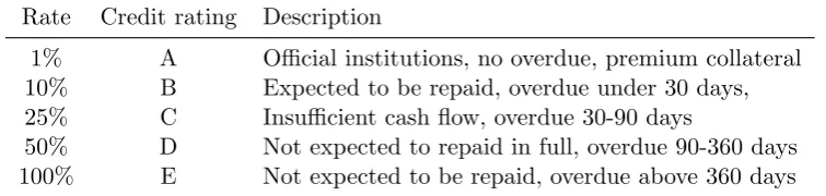
Before 2006, provisioning rates were set by the Bank of Slovenia. It set them based on historical
data in a conservative manner. Provision and impairment rates applicable before 2006 are presented
in Table 1. When the bank issued a loan, it immediately impaired the carrying amount in line with
risk buckets presented in Table 1. If a loan was downgraded to a higher risk bucket, the bank had
[image:8.595.110.488.319.409.2]to apply higher provision rate irrespective if the loss has not materialized.
Table 1: Provision and impairment rates valid in Slovenian banking sector before 2006
Rate Credit rating Description
1% A Official institutions, no overdue, premium collateral 10% B Expected to be repaid, overdue under 30 days, 25% C Insufficient cash flow, overdue 30-90 days
50% D Not expected to repaid in full, overdue 90-360 days 100% E Not expected to be repaid, overdue above 360 days
Source: Provision or impairment rates can be found in The Official Gazzete of the Republic of Slovenia (2005, No. 67a), article 22. Definitions of asset classes can be found in the same document, under article 11.
In 2006, Slovenian banks traversed to IFRS. Under the IFRS the provision and impairment
rates were no longer set by the Bank of Slovenia, but were set by banks themselves using fair
value approach. Many banks kept the system of assigning provisions based on credit ratings. But,
importantly, banks were now free to determine provisioning rates for each risk bucket. They no
longer applied those presented in Table 1.
On average, the historical approach imposed higher provision and impairment rates than the fair
value approach. Under the fair value approach a bank is required to provision for losses related to
materialized events. In contrast, under the historical approach the loan loss provisions are recorded
regardless if the losses have materialized or not.
The Bank of Slovenia foresaw that the amount of provisions and impairments will decrease under
the IFRS (see Bank of Slovenia (2015)). A substantial decrease of provisions and impairments would
increase bank profit at that time, which could be paid out in dividends, making banks less capitalized
To prevent capital outflow, the Bank of Slovenia amended rules on credit risk calculation8
and
the regulation on bank capital calculation9
. The amendments stated that, for regulatory purposes,
the banks were required to introduce a (own funds) deduction item10
. It was named prudential
filter and was calculated as the difference between provisions and impairments calculated by using
the historical approach rates and the provisions and impairments calculated under the fair value
approach. This rule applied only to loans and claims that were provisioned collectively under the
IFRS. Individually impaired loans, which are to a large extent non-performing loans, were exempt
from this calculation, since for these loans the bank thoroughly assesses the expected cash flow and
provision accordingly.
Since the prudential filter was deducted from Tier I capital, it forced banks to hold higher capital
from 2006q1 to 2008q3. This approximated the effect of a counter-cyclical buffer if it existed at the
time.
On several occasions banks requested to abdicate the prudential filter. That would make banks
more profitable per unit of capital, but also less resilient to future shocks. The Bank of Slovenia
declined their requests and only removed the prudential filter in 2008q4, at the first signs of financial
crisis. As a direct impact of the abolishment of the prudential filter, the bank capital adequacy ratio
increased, on average by 0.8 percentage points. Sudden increases in bank capitalization implied that
banks could use excess capital for either lending or credit loss absorption. This is exactly what the
counter-cyclical capital buffer is designed for.
The functioning of the prudential filter is presented in Figure 2. The dashed line shows the
amount of the prudential filter, which was about 0.8% of RWA before the release and zero afterwards.
The capital adequacy ratio (solid line in Figure 2) displays a mirrored picture. It increased when
the prudential filter was released. The prudential filter increased capital requirements during an
expansionary period and alleviated them in time of crisis.
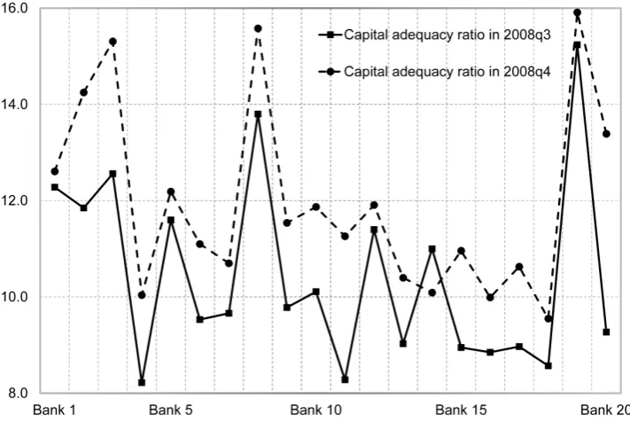
Figure 3 shows the capital adequacy ratio by banks before and after the release. The prudential
filter caused an increased in the CAR for all banks except one. Note the difference between the
dashed and solid line in Figure 3. It does not arise only due to a prudential filter release. There
might have been other factors influencing the change in the CAR between 2008q3 and 2008q4, say
recapitalization or realization of losses. This explains a decrease in the CAR for the one bank, which
8
See The Official Gazzete of the Republic of Slovenia (2005, No. 67a).
9
See The Official Gazzete of the Republic of Slovenia (2005, No. 67b).
10
Figure 2: Weighted Mean of CAR and Prudential Filter in % of RWA, 2007-2010
Source: Bank of Slovenia, own calculations.
could not arise due to the prudential filter release. The prudential filter can only increase capital
available to a bank.
Figure 3: CAR before the release (2008q3) and after it (2008q4), across banks
Source: Bank of Slovenia, own calculations.
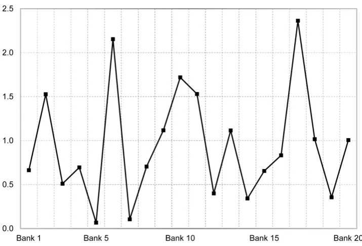
Pure effects of the prudential filter release on capital adequacy ratio is depicted in Figure 4.
[image:10.595.118.474.442.680.2]RWA. This is our main policy variable. We use it in a loan level model to test if banks with a
higher amount of prudential filter lent and provisioned by more at the beginning of the crisis. Our
identification strategy (described in Section 3.1) demands that prudential filter varies across banks.
This enables us to estimate the effect of a 1 p.p. increase in capital buffer on bank lending, while
controlling for loan demand11
. Fortunately, it does vary across banks. Nine banks had a prudential
filter that was above 1% of RWA. Nine banks had values within a band of 0.3-1% and two banks
held a prudential filter that was close to 0%. These amounts translated to an increase in capital
[image:11.595.116.474.269.512.2]adequacy at the time of prudential filter release.
Figure 4: Prudential Filter in 2008q3 in % of RWA, across banks
Source: Bank of Slovenia, own calculations.
There is a conceptual difference between the prudential filter and the CCyB. Under the CCyB
the rate of additional capital is same for all banks (up to 2.5% of RWA). On the other hand,
prudential filter was bank specific. It ranged from close to 0% of RWA to 2.4% of RWA. The fact
that the prudential filter varied facilitates our analysis. For this reason we estimate the average
effect of a 1 p.p. increase in the capital buffer. Note also that the CCyB is applied by increasing the
minimum capital requirement whereas prudential filter decreased the accounting value of capital
that entered the calculation of capital adequacy ratio. Regardless, in practice they both increase
11
If each bank-firm pair had the same amount of prudential filter we could not exploit the differences-in-differences
approach. The difference would always be zero. If we could not exploit the differences-in-differences approach we
capital available to banks at the time of capital release.
3
Methodology
We now present the identification strategy and data used to estimate the effect of the capital buffer
release on bank lending and loan loss provisioning.
3.1 Identification Strategy
In this section we describe the identification strategy employed in the loan level model. Its key
advantage is that it controls for loan demand and thereby yields unbiased and consistent estimates
of coefficients. Methodology used in this section was put forward by Khwaja and Mian (2008). It
was further adopted by Jim´enez et al. (2010), Jim´enez et al. (2017), Bonaccorsi di Patti and Sette
(2016), Behn et al. (2016) and others.
Khwaja and Mian (2008) use a clever estimation technique that allows one to control for loan
demand. It is an unobserved variable12
. This implies that any model explaining credit growth is
missing a key control variable. If this variable is correlated with other regressors, the coefficients
are biased and inconsistent. The extent of bias depends on the degree of its correlation with the
variable that we are vested in. A possible way of controlling for loan demand is to introduce a proxy
for loan demand, such as real GDP or investment. But unfortunately, the degree of bias will remain
unknown.
Khwaja and Mian (2008) bypass this issue by exploiting loan level data. In their setting, loan
level data are data on borrowers with (at least) two banking relations. The idea is simple. If
in a given period the borrower’s loan demand is constant over two banks, then we can introduce
a borrower specific dummy that controls for loan demand. An analogous approach is used in a
fixed effects model by means of transforming the data over the time dimension13
. The next few
12
Only in rare instances is the researcher endowed with loan applications data which are an excellent proxy for loan
demand. See for example Jim´enez et al. (2012).
13
By employing either a dummy variable estimator, within, between or the fixed effects transformation. Note the
subtle difference between the fixed effects estimator and the Khwaja and Mian (2008) difference-in-difference estimator.
The fixed effects estimator exploits the fact that the fixed effects are constant over time. With at least two time periods
of observations they can be controlled for using a dummy for each borrower or by means of data transformation. This
works similarly also in our case, the only difference being that instead of time the second dimension that determines
paragraphs present a simplified example that explains the idea originally put forward by Khwaja
and Mian (2008).
Suppose that we haveN borrowers with at least two banking relations in a given time period14
:
yij =βXij+ηi+ǫij (1)
Where yij stands for borrower i’s loan growth (where i = 1...N) in bank j (where j = 1...M) in
specific time period around the filter release. The period is defined in Section 3.2. Xij represents a
K×1 vector of policy and control variables that we don’t specify further at this point. ηi represents
firm-level effects that can not be observed by the researcher. The key firm-level unobserved effect
in our model is loan demand. Suppose we now add to eq. (1) a dummy variable that takes the
value of 1 for individualiand zero elsewhere15
. Becauseηi is invariant between banks (j = 1...M),
it will be absorbed by the dummy variable:
yij =βXij +Di+ǫij (2)
Since Di is equal to one for all banks it absorbs firm demand and all other firm characteristics.
The observed effect can thus be fully attributed to the differences between banks. In our case this
means that the estimated effect of prudential filter release on credit growth, presented in the next
section, can be attributed to differences in banks loan supply related to different levels of prudential
filter.
We use the same approach to estimate the effect of a buffer release on bank loan loss provisioning.
The dependent variable in that case is a change in the coverage ratio realized by bankj for firmi.
Two key factors determining the rate of provisioning are firm riskiness and the amount of collateral.
While both variables can in general be observed, our loan level methodology is still advantageous.
It captures all firm-level effects, including riskiness and availability of collateral. We address other
potential firm-bank specific issues in Section 4.
14
This is a reduced form model. Khwaja and Mian (2008) derived it from a simplified theoretical model.
15
The estimator of such model is called the least squares dummy variable estimator. If the number of borrower’s
(N) is large one can use transformations of the data (like for instance within transformation) that cause the fixed
3.2 Data
We use data from the credit register of the Bank of Slovenia. It contains multiple observations for
each borrower in each time period. This is necessary for our identification methodology described
in the previous section. Loans on a borrower level are available only for firms. Households loans
are reported only cumulatively across risk buckets and can not be used with our loan level model.
By considering only corporate loans we still capture majority of total loan volume to private
non-financial sector. Loans to households represented only 23% of credit to private non-non-financial sector
in 2008.16
The first important step in data preparation is to select an appropriate period to be used in
credit growth calculation. Our baseline period is credit growth in the period between one quarter
before prudential filter release (2008q3) and three quarters after the release (2009q3). One could
argue that this selection is rather subjective. We also estimate the model on horizons from 1 to 4
quarters after the release and report on those results.
We exclude firms with missing values. For identification purposes we restrict our sample to firms
that are indebted to at least two banks. After imposing this restriction we are left with 7,882 firms.
They account for 22.3% of all the firms that were in the same period indebted to at least one bank.
Admittedly, this share is low, however, their total loan amount is equal to 84.2% of loans. Thus the
data is representative and covers a large share of the total amount of loan to firms. Firms indebted
to multiple banks are typically larger and hold bigger loan amounts. Next, for estimating the effect
of buffer release on lending, we restrict our sample to performing firms only. We exclude the
non-performing firms because accounting rules dictate that non-paid interest on NPLs have to be added
to the amount of non-performing loans. Increase of the the loan amount is caused by accounting
regulation and could be spuriously correlated with our regressors. Lastly, to eliminate outliers, we
exclude firms of the 1st and 100th percentile of the distribution of our dependent variables.
In estimating the effect on loan loss provisioning we focus on firms that are either in default or
have difficulties in repaying the loan. Only these need to be provisioned extensively and account for
16
We also performed aggregate analysis where also loans to households were included. We estimated the bank level
dynamic panel-data model where the dependent variable is loan growth to firms and households. The results are in
line with the findings presented in Section 4. The estimated effect of buffer release on bank lending is however lower,
which can be attributed to the lack of control for loan demand in the bank level model, different sample and different
estimation methodology. The results are available upon request. We do not report on them because of the potential
the majority of loan loss reserves. Including the performing firms we would find a much smaller or
maybe even no effect on provisions. The reason being that there is no need to provision additionally
for firms that repay their loan regularly. This follows from the IFRS incurred loss provisioning
model. Similarly as in the case of loan growth analysis we eliminate outliers.
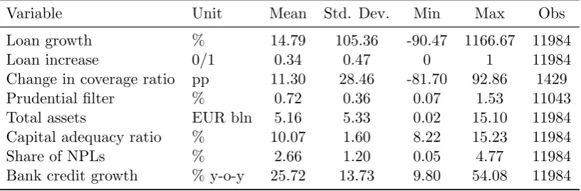
Table 2 shows summary statistics for the variables included in the model. Credit growth is
calculated as a percentage growth comparing one quarter before release and three quarters after the
buffer release (2008q3 to 2009q3). Mean credit growth is 15%. Loan increase is a dummy variable
equal to 1 if firmi’s loan amount increased in bankj in the period 2008q3-2009q3. 34% of the firms
increased their indebtedness after the release. The second variable of interest is change in coverage
ratio. It has a mean equal to 11.3 p.p.17
It is calculated only for the non-performing firms. All
policy and control variables are included in the model at their values in 2008q3, i.e. just before the
release. The average value of our main policy variable, the prudential filter, was 0.72%18
in 2008q3.
Bank size is measured by total assets. Its average value in 2008q3 was about EUR 5 bln. Average
capital adequacy ratio, share of non-performing loans and y-o-y bank credit growth before the filter
[image:15.595.95.503.425.559.2]release were 10.1%, 2.7% and 25.7%, respectively.
Table 2: Summary Statistics
Variable Unit Mean Std. Dev. Min Max Obs
Loan growth % 14.79 105.36 -90.47 1166.67 11984
Loan increase 0/1 0.34 0.47 0 1 11984
Change in coverage ratio pp 11.30 28.46 -81.70 92.86 1429 Prudential filter % 0.72 0.36 0.07 1.53 11043 Total assets EUR bln 5.16 5.33 0.02 15.10 11984 Capital adequacy ratio % 10.07 1.60 8.22 15.23 11984 Share of NPLs % 2.66 1.20 0.05 4.77 11984 Bank credit growth % y-o-y 25.72 13.73 9.80 54.08 11984
Source: Bank of Slovenia, own calculations.
Notes: Loan growth is calculated for the period 2008q3-2009q3. Credit increase is a dummy variable equal to 1 if firmiloan amount increased in bankjin period 2008q3-2009q3. Prudential filter, total assets, capital adequacy ratio, share of NPLs and Bank credit growth are reported at their values from 2008q3, just before the release took place. Change in coverage ratio is calculated for defaulted firms, whereas all other statistics are reported for performing part of the sample.
4
Results
This section presents the results. We investigate if banks with a higher amount of a prudential filter
and a higher capital adequacy lent more at the beginning of the crisis. Next, we verify the nature
17
Change in coverage ratio is calculated as ∆CRij=
P rovisionsij,2009q3
Loansij,2009q3 −
P rovisionsij,2008q3
Loansij,2008q3 .
18
of firms the additional lending was directed to. Lastly, we verify if banks used spare loss-absorption
capacity, that occurred with capital release, to provision more for bad loans. By answering these
questions, we can test whether the policy of a capital buffer release in bad times is effective and if
it serves its main goals.
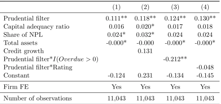
Table 3 shows the effect of buffer release on bank lending.19
Dependent variable is firm’sicredit
growth on a loan taken with bankj in period 2008q3-2009q3. We control for firm specific demand
with firm-fixed effects and include several controls for other influences. Model (1) in Table 3 shows
our baseline results. We find that for the same firm, borrowing from at least two different banks
that differ in the size of prudential filter, credit growth was 11.1 p.p. higher if the bank had a 1
p.p. higher capital buffer. By using standard errors clustered at the bank level, this coefficient
is statistically significant at conventional levels. This implies that a capital buffer release indeed
[image:16.595.116.482.359.532.2]increased bank lending.
Table 3: The Effect of Capital Buffer Release on Bank Lending
(1) (2) (3) (4)
Prudential filter 0.111** 0.118** 0.124** 0.130** Capital adequacy ratio 0.016 0.020* 0.017 0.018 Share of NPL 0.024* 0.032* 0.024 0.024 Total assets -0.000* -0.000 -0.000* -0.000*
Credit growth 0.131
Prudential filter*I(Overdue >0) -0.212**
Prudential filter*Rating -0.048
Constant -0.124 0.231 -0.134 -0.145
Firm FE Yes Yes Yes Yes
Number of observations 11,043 11,043 11,043 11,043
Source: Bank of Slovenia, own calculations.
Notes: The table reports the estimation results for loan level differences-in-differences model. Dependent variable in all the equations is firmiloan growth in bankj in period 2008q3-2009q3 (10% is expressed as 0.1). Prudential filter is its amount in 2008q3 (just before the release), expressed in percent of RWA. Capital adequacy ratio, share of NPL and bank total assets are taken from 2008q3. Credit growth is bank specific credit growth in year before prudential filter release. I(Overdue >0) is an indicator equal one if firm i
repays the loan to bankjwith overdue higher than zero days. Rating is a credit rating as-signed by bankjto firmiand takes values from 0 (rating A) to 4 (rating E). Significance: *p <0.10, **p <0.05, ***p <0.01.
We now extend our baseline model with a bank’s credit growth in the year prior to prudential
filter release. If banks that held a higher amount of prudential filter are the banks that lent more
before the capital release then the identified effect could be incorrectly attributed to the prudential
19
filter release. It might only reflect a higher credit growth of banks that incidentally held a high
amount of prudential filter. As shown in model (2) in Table 3 this is not the case. Even when
controlling for a bank’s credit growth, the prudential filter displays a positive and statistically
significant effect. In addition, the effect of bank credit growth before the release of capital is found
insignificant.
Our next set of results investigates which firms benefited from the positive effect of the filter
release. Note that this was the period when the crisis began and non-performing loans started to
accumulate in bank balance sheets. Banks may engage in the evergreening of loans to riskier firms.
They do this to reduce the pressure of loan-loss provisions on capital. This phenomenon is well
documented by Peek and Rosengren (2005). If the capital buffer amplifies this effect that would be
undesirable.
To verify this, we interact prudential filter with two variables that measure firm riskiness. The
delay with which firm i repays debt to bankj is an indicator of risk. Model (3) in Table 3 shows
this result. The interaction term is negative. In addition, the sum of the coefficients for a prudential
filter and the interaction term is also negative. This implies that the positive effect of the prudential
filter release is not only reduced for borrowers that have difficulties with loan repayment, but is even
negative. The credit rating assigned by bank j to firmi is our second measure of risk. It takes a
value from zero (rating A) to four (rating E). The coefficient on the interaction term is negative,
though it is not statistically significant (exact p-value is equal to 0.153). Overall, we conclude that
solid and safe firms gain the most from a capital buffer release. This is a desirable outcome for
policy makers.
The results presented indicate a possible impact of a capital buffer release on loan growth for a
specific time horizon, 2008q3-2009q3. To verify the robustness of this result we present regression
results based on different periods. So far, we have used 2008q3 as a cut-off date before the prudential
filter is released. We would like to stay as close as possible to the time of the buffer release so we
do not contaminate the dependent variable with other effects. For the same reason we also don’t
look any further beyond 1 year after the release.
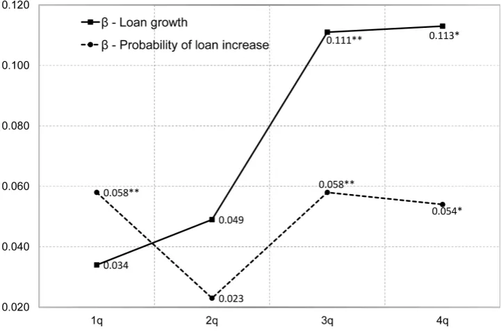
Figure 5 presents the results for horizons that span from 1 to 4 quarters after the release. The
effect of capital release on loan growth peaked in the third quarter after the release. Importantly,
the estimated coefficient is positive in all the cases. It is, however, statistically significant only for
the third and fourth quarter after the release. This is to some extent expected, since banks typically
[image:18.595.117.478.156.396.2]need some time to re-allocate spare capital.
Figure 5: Coefficient for loan growth and for the probability of a loan increase on one- to four-quarter horizon after the release
Source: Bank of Slovenia, own calculations. Significance: *p <0.10, **p <0.05, ***p <0.01.
We also estimate the probability of a loan increase based on the release of a prudential filter.
The dependent variable is equal to 1 if firmi’s amount of loan borrowed from bank j has increased
in the period. We use the same time horizon as in our benchmark regression. The advantage of
this approach is that the estimated effects are not driven by outliers, which are, despite certain
exclusions, still quite high. The results are presented in Figure 5. Comparable to credit growth, we
find that release of the capital buffer increases the probability of a loan growth. We find that a firm
had a 5.8 p.p. higher probability of a loan increase with a bank that held a 1 p.p. higher capital
buffer.
We now explore the effect of capital release on bank loan loss provisioning. Due to a filter release
banks obtained spare capital that increased their loss absorption capacity. A study by
Brezigar-Masten et al. (2015) shows that banks intentionally underestimated credit risk in response to an
increase in non-performing loans. We test if banks with higher capital buffers provisioned more,
thereby ameliorating underestimation of credit risk.
each observation between 2008q3 and 2009q3. We control for firm fixed effects. We focus on firms
that are either in default or are in overdue. We present three different sets of results differing in
[image:19.595.86.511.160.338.2]firm’s overdue.
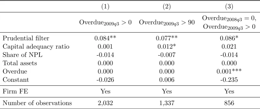
Table 4: The Effect of Capital Buffer Release on Bank Loan Loss Provisionig
(1) (2) (3)
Overdue2008q3 = 0,
Overdue2009q3>0 Overdue2009q3 >90
Overdue2009q3 >0
Prudential filter 0.084** 0.077** 0.086* Capital adequacy ratio 0.001 0.012* 0.021
Share of NPL -0.014 -0.007 -0.014
Total assets 0.000 0.000 0.000
Overdue 0.000 0.000 0.001***
Constant -0.026 0.006 -0.235
Firm FE Yes Yes Yes
Number of observations 2,032 1,337 856
Source: Bank of Slovenia, own calculations.
Notes: The table reports the estimation results for the loan-level differences-in-differences model. The dependent variable in all the equations is the change in loan loss provisioning ratio between 2008q3 and 2009q3. Model is estimated for three subsamples: (1) and (2) includes firms that had overdue higher than 0 and 90 days, respectively, whereas (3) includes firms that were in overdue after buffer release conditional of not being in overdue before. Prudential filter is recorded at its amount in 2008q3 (just before the re-lease) and expressed in percent of RWA. Capital adequacy ratio, share of NPL and bank total assets are taken from 2008q3. Overdue controls for specific firm i’s overdue in bankj. Significance: *p <0.10, **
p <0.05, ***p <0.01.
We find that the prudential filter release increased loan loss provisioning. Model (1) in Table 4
shows the results for the sample of firms that were past due with loan repayment in 2009q3 for at
last one day. For the same firm the coverage ratio increased by 8.4 p.p. more in banks that held a
1 p.p. higher capital buffer. Next, we use a more strict criteria in sample selection and include only
firms that were more than 90 days overdue. This threshold is typically used to classify borrowers
as non-performing, so banks provision extensively only after it is bridged. The results, presented in
column (2), confirm our previous findings. One might be concerned that for the majority of firms
included in models (1) and (2) the coverage ratio is constant because they were in default for a long
time and had been provisioned accordingly. This might indeed be the case. The average number of
days overdue among defaulted firms is above 500 days. To address this issue we estimate a model
for firms that became past due after the prudential filter abdication. They are new defaulters that
banks provisioned for the first time after capital release. The results are shown in column (3) in
Table 4. We find a positive effect that is similar in magnitude to our previous result. We re-confirm
We now address some firm-bank specificities that could influence our finding of increased
provi-sioning. The longer the time in default the higher should be the coverage ratio, all else being equal.
Firms, however, do not start to delay with loan repayment to all banks at the same time. There
might be difference in the coverage ratio for the same firms across multiple banks. To address this
we add overdue-in-loan-repayment as a control variable. For models (1) and (2) it is irrelevant.
The reason for this is that the difference in overdue of 10 or 50 days is negligible for firms that
have already been in overdue for a long time. Once the number of days in overdue becomes high,
banks estimate that it is unlikely that a loan will be repaid and they provision accordingly. For
new defaulters in model (3), however, this variable is found to be relevant. A firm that started to
delay loan repayment with bankA 50 days before it started to delay loan repayment with bankB,
is expected to have on average a 5 p.p. higher coverage ratio in bankA as compared to bankB.
The second determinant of loan loss provisioning is collateral. Omission of collateral is to some
degree controlled for with fixed effects. They capture the total firm’s collateral. Banks, however,
differ in strategy and ability to engage a firm’s collateral. Unfortunately, we cannot control for the
exact amount of collateral pledged by firm i in bankj. These data are not available. We instead
asses the direction of bias assuming the collateral does affect loan loss provisioning.
The bias depends on the correlation between provisioning, collateral and the prudential filter.
First, we establish that the prudential filter and collateral are positively correlated by excluding
a negative one. Banks that held a higher filter also held lower collateral. We know that banks with
a higher filter suffered smaller losses in the period 2009-2014.20
Lower losses imply that those banks
held more and better collateral. It is reasonable to assume that banks with a higher filter held more
or better collateral. This implies the filter and collateral were positively correlated.
Next, we know that collateral and loan loss provisions are negatively correlated. This follows
from basic accounting rules. Had loans been fully collateralized, there would be no need for
provi-sions.
Finally, we determined that our omitted variable (collateral) is negatively correlated with the
dependent variable (loan loss provisions) and positively correlated with our target variable
(pru-dential filter). Therefore, if a pru(pru-dential filter acts as a proxy for collateral, the coefficient will be
downward biased. Our estimates of the effect of the capital buffer on provisioning represent a lower
boundary on the coefficient estimate.
20
The correlation between total bank losses in the period 2009-2014 expressed as a share of pre-crisis assets and the
5
Conclusion
This paper studies a unique experiment in the Slovenian banking system in 2007-2010. The
ex-periment is called the prudential filter and it acted like a countercyclical capital buffer. In 2008q4,
an exogenous shock caused the prudential filter abdication. It increased capital by 0.8% of
risk-weighted assets. We estimate how this release of capital, akin to a countercyclical capital buffer,
affected the banking system at the start of the financial crisis.
In 2006, Slovenian banks adopted IFRS. This led to a change in the way loan loss provisions
and impairments were calculated. Fearing that the new method would decrease loan provisions,
the Bank of Slovenia introduced a prudential filter. It was calculated as the difference between
provisions and impairments calculated under the IFRS and the old Slovenian Reporting Standards
rules. The prudential filter was used as a deduction from capital in the calculation of bank’s capital
adequacy ratio. The deduction item forced banks to hold more capital. The prudential filter was
abdicated at the start of the financial crisis in Slovenia in 2008q4. Following its release the capital
ratio of the banking system increased by 0.8 percentage point.
The prudential filter is similar in nature to a countercyclical buffer. It accumulated bank capital
in times of excess credit growth and released it at the start of the crisis. Our study contributes to
the literature on the countercyclical capital buffer by providing empirical results of a situation akin
to a release of countercyclical capital buffer.
We investigate the effects of the release of the prudential filter on credit growth using loan-level
data from the Slovenian credit register. We find that three quarters after the release, credit growth
for the same firm, borrowing from at least two different banks, was on average 11 p.p. higher in
a bank that had a 1 p.p. higher capital buffer. This result is robust to model specifications and
the credit growth horizon. It suggests that the CCyB, which is designed to smooth credit growth,
increased credit at the start of the crisis.
The second finding is that solid firms benefit most from the buffer release. This is important
information for policymakers and banking regulators. It shows that by releasing the capital buffer,
banks channel the new crediting capacity to healthy firms. They act countercyclical. This intensifies
the positive effect of the buffer on the real economy.
Finally, banks use an additional loss-absorption-capacity that arises with a buffer release, to
provision more for defaulted borrowers. This is a desired result since a delay in loan-loss recognition
Our investigation provides empirical support in favor of the effectiveness of capital based
macro-prudential instruments.
References
David Aikman, Benjamin Nelson, and Misa Tanaka. Reputation, risk-taking, and macroprudential
policy. Journal of Banking & Finance, 50:428–439, 2015.
Q. Farooq Akram. Macro effects of capital requirements and macroprudential policy. Economic
Modelling, 42:77–93, 2014.
Bruce Arnold, Claudio Borio, Luci Ellis, and Fariborz Moshirian. Systemic risk, macroprudential
policy frameworks, monitoring financial systems and the evolution of capital adequacy. Journal
of Banking & Finance, 36(12):3125–3132, 2012.
Christoph Carl Basten and Catherine Koch. Higher bank capital requirements and mortgage pricing:
evidence from the countercyclical capital buffer (CCB). Technical report, BIS Working Paper No
511, 2015.
BCBS. Basel III: A global regulatory framework for more resilient banks and banking systems.
Technical report, Basel Committee on Banking Supervision, Basel, 2010.
BCBS. Frequently asked questions on the basel III countercyclical capital buffer. Technical report,
Basel Committee on Banking Supervision, Basel, 2015.
Anne Beatty and Scott Liao. Do delays in expected loss recognition affect banks willingness to
lend? Journal of Accounting and Economics, 52, 2011.
Marcus Behn, Rainer Haselmann, and Paul Wachtel. Procyclical capital regulation and ledning.
Journal of Finance, 71:919–956, 2016.
Crisitina Biu, Harald Scheule, and Eliza Wu. The value of bank capital buffers in maintaining
financial system resilience. Journal of Financial Stability, 33:23–40, 2017.
Emilia Bonaccorsi di Patti and Enrico Sette. Did the securitization makret freeze affect bank lending
during the financial crisis? Evidence from a credit register. Journal of Financial Intermediation,
Arjana Brezigar-Masten, Igor Masten, and Matjaˇz Volk. Discretionary credit rating and bank
stability in a financial crisis. Eastern European Economics, 53(5):377–402, 2015.
Micha l Brzoza-Brzezina, Marcin Kolasa, and Krzysztof Makarski. Macroprudential policy and
imbalances in the euro area. Journal of International Money and Finance, 51:137–154, 2015.
Eugenio Cerutti, Stijn Claessens, and Luc Laeven. The use and effectiveness of macroprudential
policies: new evidence. Journal of Financial Stability, 28:203–224, 2017.
Stijn Claessens. An overview of macroprudential policy tools. Technical report, IMF Working Paper,
14/214, 2014.
Gabriele Galati and Richhild Moessner. Macroprudential policy: a literature review. Journal of
Economic Surveys, 27(5):846–878, 2013.
Hans Gersbach and Jean-Charles Rochet. Capital regulation and credit fluctuations. Journal of
Monetary Economics, 2017.
Marco Gross, Christoffer Kok, and Dawid ˙Zochowski. The impact of bank capital on economic
activity-evidence from a mixed-cross-section gvar model. Technical report, ECB Working Paper
Series 1888, 2016.
Timotej Homar and Sweder van Wijnbergen. On zombie banks and recessions after systemic banking
crises. Technical report, CEPR Discussion Papers 10963, 2015.
Maria Iosifidi and Sotirios Kokas. Who lends to riskier and lower-profitability firms? evidence from
the syndicated loan market. Journal of Banking & Finance, 61:S14–S21, 2015.
Gabriel Jim´enez, Atif R Mian, Jos´e-Luis Peydr´o, and Jes´us Saurina. Local versus aggregate lending
channels: the effects of securitization on corporate credit supply in spain. Technical report,
National Bureau of Economic Research, 2010.
Gabriel Jim´enez, Steven Ongena, Jos´e-Luis Peydr´o, and Jes´us Saurina. Credit supply and
mone-tary policy: Identifying the bank balance-sheet channel with loan applications. The American
Economic Review, 102(5):2301–2326, 2012.
Gabriel Jim´enez, Steven Ongena, Jos´e-Luis Peydr´o, and Jesus Saurina Salas. Macroprudential
policy, countercyclical bank capital buffers and credit supply: Evidence from the spanish dynamic
Mahdi Ebrahimi Kahou and Alfred Lehar. Macroprudential policy: A review. Journal of Financial
Stability, 29:92–105, 2017.
Asim Ijaz Khwaja and Atif Mian. Tracing the impact of bank liquidity shocks: Evidence from an
emerging market. The American Economic Review, pages 1413–1442, 2008.
Joseph Noss and Priscilla Toffano. Estimating the impact of changes in aggregate bank capital
requirements on lending and growth during an upswing. Journal of Banking & Finance, 62:
15–27, 2016.
Bank of Slovenia. Report of the BoS on the causes of the capital shortfalls of banks and the role
of the Bank of Slovenia as the banking regulator in relation to the recovery of banks in 2013 and
2014. Technical report, 2015.
Official Gazette of the Republic of Slovenia. Regulation on the assesment of credit risk losses of
banks and savings banks. Technical report, 2005, No. 67a.
Official Gazette of the Republic of Slovenia. Regulation on the assesment of credit risk losses of
banks and savings banks. Technical report, 2005, No. 67b.
Official Gazette of the Republic of Slovenia. Regulation on the assesment of credit risk losses of
banks and savings banks. Technical report, 2015, No. 50.
Joe Peek and Eric S. Rosengren. Unnatural selection: Perverse incentives and the misallocation of
credit in japan. The American Economic Review, 95(4):1144–1166, 2005.
Margarita Rubio and Jos´e A Carrasco-Gallego. The new financial regulation in basel III and
monetary policy: A macroprudential approach. Journal of Financial Stability, 26:294–305, 2016.
William J Tayler and Roy Zilberman. Macroprudential regulation, credit spreads and the role of