A Convex Optimisation Approach
to Optimal Control in Queueing Systems
V´ıctor Valls
School of Computer Science and Statistics Trinity College Dublin
Submitted for the Degree of Doctor of Philosophy Supervised by Prof. Douglas Leith
Abstract
Convex optimisation and max-weight are central topics in networking and control, and having a clear understanding of their relationship and what this involves is crucial from a theoretical and practical point of view. In this thesis we investigate how max-weight fits into convex optimisation from a pure convex approach without using fluid limits or Lyapunov optimisation. That is, we study how to equip convex optimisation with discrete actions and allow it to make optimal control decisions without previous knowledge of the mean packet arrival rate into the system.
Our results are sound and show that max-weight approaches can be encompassed within the body of convex optimisation. In particular, max-weight is a special case of the stochastic dual subgradient method withǫk-subgradients and constant step size. We clarify
the fundamental properties required for convergence, and bring to the fore the use of ǫk
-subgradients as a key component for modelling problem characteristics apart from discrete actions. One of the great advantages of our approach is that optimal scheduling policies can be decoupled from the choice of convex optimisation algorithm or subgradient used to solve the dual problem, and as a result, it is possible to design scheduling policies with a high degree of flexibility. We illustrate the power of the analysis with three applications: the design of a traffic signal controller; distributed and asynchronous packet transmissions; and scheduling packets in networks where there are costs associated to selecting discrete actions.
Acknowledgements
A special thank you to my supervisor, Prof. Doug Leith, for his guidance and support during these four years. I feel fortunate to have had him as a supervisor; his vibrant approach to research has made a big impact on me on a professional and personal level. I would also like to thank Dr. Xavier Costa for giving me the opportunity to visit the NEC Laboratories in Heidelberg, and Prof. Boris Bellalta for his guidance during the early stages of my career.
Thanks also to all my friends in Ireland, Germany, and Spain. To my friends and col-leagues at Trinity College and the Hamilton Institute: Cristina Cano, Alessandro Checco, Saman Feghhi, Andr´es Garc´ıa-Saavedra, Naoise Holohan, Mohammad Karzand, Julien Monteil and Giulio Prevedello; to my friends in Mannheim, Tim Schneider and Vita Spanier, without whom I would have not had so much fun during my time in Germany; and to all my friends in Girona and Barcelona that are too many to list, but hope to see very soon.
Finally, I would like to thank my brother and parents for all their support and love.
My doctoral studies have been supported by Science Foundation Ireland under Grant No. 11/PI/1177.
Contents
Abstract . . . ii
Acknowledgements . . . iii
Chapter 1. Introduction . . . 1
1.1. Purpose of the Thesis . . . 2
1.2. Contributions . . . 3
1.3. Notation . . . 5
1.4. Related Work . . . 5
1.5. Thesis Outline . . . 8
Chapter 2. Sequences of Non-Convex Optimisations . . . 10
2.1. Preliminaries . . . 10
2.2. Non-Convex Descent . . . 12
2.2.1. Non-Convex Direct Descent . . . 12
2.2.2. Non-Convex Frank-Wolfe-like Descent . . . 16
2.3. Constrained Convex Optimisation . . . 19
2.3.1. Lagrangian Penalty . . . 19
2.3.2. Non-Convex Dual Subgradient Update . . . 20
2.3.3. Generalised Update . . . 28
2.4. Using Queues as Approximate Multipliers . . . 28
2.4.1. Weaker Condition for Loose Constraints . . . 33
2.4.2. Queue Stability . . . 33
2.4.3. Optimal Actions Depend Only on Queue Occupancy . . . 33
2.5. Max-Weight Revisited . . . 34
2.6. Numerical Example . . . 35
Chapter 3. Dual Subgradient Methods with Perturbations . . . 38
3.1. Dual Subgradient Methods . . . 38
3.1.1. Classic Dual Subgradient Method . . . 39
3.1.2. Computing a Subgradient of the Lagrange Dual Function . . . 41
3.1.3. Stochastic Dual Subgradient Methods . . . 43
3.2. Bounded Lagrange Multipliers and Feasible Solutions . . . 46
3.3. Framework . . . 46
3.3.1. Parameterised Problem Setup . . . 47
3.3.2. Dual Subgradient Method with Perturbations . . . 48
3.3.3. Convergence . . . 52
Chapter 4. Actions and Asynchronous Updates . . . 60
4.1. Preliminaries . . . 60
4.1.1. Problem and Action Set . . . 60
4.1.2. Discrete Actions and Approximate Lagrange Multipliers . . . 61
4.2. Asynchronous Dual Updates . . . 62
4.2.1. Dual Decomposition . . . 63
4.2.2. Asynchronous Updates . . . 64
4.3. Sequences of Non-Convex Actions . . . 66
4.3.1. Blocks of Discrete Actions . . . 66
4.3.2. Online Sequences of Discrete Actions . . . 71
Chapter 5. Applications . . . 76
5.1. Traffic Signal Control . . . 76
5.1.1. Preliminaries . . . 78
5.1.2. Convex Optimisation Approach . . . 80
5.1.3. Numerical Example . . . 85
5.2. Distributed and Asynchronous Packets Transmissions . . . 91
5.2.1. Problem Setup . . . 91
5.2.2. Simulation . . . 92
5.3. Packet Transmissions with Constraints . . . 94
5.3.1. Problem Setup . . . 95
5.3.2. Simulations . . . 96
Chapter 6. Conclusions . . . 98
Appendix A. . . 99
CHAPTER 1
Introduction
Convexity plays a central role in mathematical optimisation from both a theoretical
and a practical point of view. Some of the great advantages of formulating a problem as a
convex optimisation is that there exist numerical methods that can solve the optimisation
problem in a reliable and very efficient manner, and that a solution is always a global
optimum. When an optimisation problem is not of the convex type, then one enters into
the realm of non-convex optimisation where the specific structure of a problem must be
exploited in order to obtain a solution, often not necessarily the optimal one. Nevertheless,
there are some special cases of algorithms that can find optimal solutions to non-convex
problems. One is the case of max-weight scheduling, an algorithm for scheduling packets
in queueing networks which has received a lot of attention in the networking and control
communities over the last years.
In short, max-weight was proposed by Tassiulas and Ephremides in their seminal
paper [TE92]. It considers a network of interconnected queues in a slotted time system
where packets arrive in each time slot and a network controller has to make a discrete
(so non-convex) scheduling decision as to which packets to serve from each of the queues.
Appealing features of max-weight are that the action set matches the actual decision
variables (namely, do we transmit or not); that scheduling decisions are made without
previous knowledge of the mean packet arrival rate in the system; and that it is able to
stabilise the system (maximise the throughput) whenever there exists a policy or algorithm
that would do so. These features have made max-weight well liked in the community and
have fostered the design of extensions that consider (convex) utility functions, systems with
time-varying channel capacity and connectivity, heavy-tailed traffic, etc. When dealing
with utility functions, max-weight approaches usually start by formulating a fluid or convex
optimisation, and then use the solution to that problem to design a scheduler for a discrete
time system. One of the reasons for considering such an approach is that the fluid or
convex formulation provides the big picture of the problem, whereas max-weight deals
with the specific problem at a packet time scale [KY14, page 9]. Another reason used
in the literature is that the dynamics of the Lagrange multipliers (associated to linear
inequality constraints) in the dual subgradient method are like a queue update [SY13,
Section 6.1]. However, the exact nature of the relationship between these two quantities
remains still unclear, and so the body of work on max-weight approaches is separate from
the mainstream literature on convex optimisation.
The connections between max-weight and convex optimisation are of much interest
in the networking and control communities. There are several reasons for this. First, a
better understanding of the structure of the problem. Encompassing max-weight within
convex optimisation would allow us to characterise the solutions (optimality conditions)
and to exploit this to improve the performance of queueing systems. An example of this is
the work in [HN11], where the Lagrange multipliers of a convex optimisation are used to
improve the delay of a max-weight scheduler. Second, it would allow the wealth of the
well-established theory in convex optimisation to be used to bring features to max-weight that
are currently not available. For example, asynchronous updates or packets transmissions.
Third, clarity and simplicity. The popularity of max-weight has produced so many variants
of the algorithm that the state of the art is becoming increasingly complex. There is a
need for abstraction and to put concepts in a unified framework. Fourth, accessibility
and dissemination. Convex optimisation is widely used in many fields, and making
max-weight features available in convex optimisation would allow us to bring its benefits to
other areas beyond networking and control. Fifth, a new outlook. On the way to finding
the connections between max-weight and convex optimisation, we might shed light on
properties in convex optimisation that might be otherwise obscured.
1.1. Purpose of the Thesis
Convex optimisation and max-weight are central topics in networking and control,
and having a clear understanding of their relationship and what this involves is crucial.
In this thesis we investigate how max-weight fits into convex optimisation from a pure
convex approach and without invoking Foster-Lyapunov theorem. Namely, how to equip
convex optimisation with discrete actions and allow it to make optimal decisions without
knowledge of the mean packet arrival rate in the network. One of the objectives of this
thesis is to provide a concise and comprehensive approach to max-weight in the terms
used in the mainstream literature in convex optimisation [BV04, Ber99, BNO03]. That is,
in the terms that somebody familiar with dual methods in convex optimisation should be
easily able to understand. We believe that making max-weight accessible from a convex
optimisation viewpoint will help to light the way to discovering new applications currently
1.2. Contributions
(i) Generalising Max-Weight. Our analysis places max-weight firmly within the field
of convex optimisation, and rigorously shows it is a special case of the stochastic
dual subgradient method with ǫk-subgradients and constant step size. This is
shown in the optimisation framework presented in Chapter 3 in terms of
elemen-tary perturbations.
(ii) Unifying Theoretical Framework. In generalising max-weight and dual
subgradi-ent methods our analysis clarifies the fundamsubgradi-ental properties required. In
partic-ular, that the objective function and constraints need only to be convex (probably
non-differentiable); that the stochastic “noise” in the dual update must be ergodic
and have finite variance; and that theǫkperturbations on the multipliers must be
bounded. Furthermore, our analysis brings to the fore ǫk-subgradients as a key
ingredient for modelling discrete control problems, and capturing features such
as asynchronous dual updates in an easy manner.
(iii) Lagrange Multipliers, Approximate Lagrange Multipliers and Queues. We
estab-lish a clean and clear connection between queues and Lagrange multipliers. In
particular, α-scaled queue occupancies are quantities that stay close to the
La-grange multipliers in the dual subgradient method, and can be regarded as an
approximation of the true Lagrange multipliers. In some special cases α-scaled
queues are exactly Lagrange multipliers. This is first shown in Chapter 2, and
later abstracted in the form of perturbations or ǫk-subgradients in Chapter 3.
(iv) Decoupling Subgradients from Actions. By using ǫk-subgradients and the
con-tinuity of the Skorokhod map, we show that it is possible to design scheduling
policies (sequences of discrete actions) that are decoupled from a specific choice of
(sub)gradient. This is of fundamental importance because it separates the design
of scheduling policies from the characteristics of the optimisation algorithm or
type of “descent” (e.g. gradient, subgradient, newton, proximal, etc.). Another
great advantage of this approach is that it is possible to design scheduling policies
that allow some flexibility on the order in which actions can be selected, which is
key in systems that have constraints or penalties associated to selecting subsets
(v) Applications. In Chapter 5 we provide a range of examples that show the power
of the results in a concise and comprehensive manner. The examples provided
include the design of a traffic signal controller; distributed and asynchronous
packet transmissions; and scheduling of packets in networks where there are costs
associated to selecting discrete actions.
This thesis has contributed to the literature with the following publications:
• V. Valls and D. J. Leith, “A convex optimization approach to discrete optimal control,” in IEEE Transactions on Automatic Control (accepted).
• V. Valls and D. J. Leith, “Max-weight revisited: Sequences of nonconvex op-timizations solving convex opop-timizations,” in IEEE/ACM Transactions on Net-working, vol. 24, no. 5, pp. 2676-2689, Oct. 2016.
• V. Valls and D. J. Leith, “Subgradient methods with perturbations in network problems,” 54th Annual Allerton Conference on Communication, Control, and Computing (Allerton), Monticello, IL, 2016, pp. 482-487.
• V. Valls, J. Monteil and M. Bouroche, “A convex optimisation approach to traffic signal control,” IEEE 19th International Conference on Intelligent Transportation Systems (ITSC), Rio de Janeiro, Brazil, 2016, pp. 1508-1515.
• V. Valls and D. J. Leith, “Stochastic subgradient methods with approximate Lagrange multipliers,” IEEE 55th Conference on Decision and Control (CDC), Las Vegas, NV, USA, 2016, pp. 6186-6191.
• V. Valls and D. J. Leith, “Dual subgradient methods using approximate multi-pliers,” 53rd Annual Allerton Conference on Communication, Control, and Com-puting (Allerton), Monticello, IL, 2015, pp. 1016-1021.
1.3. Notation
The notation used in this thesis is a blend of the notation used in standard reference
books in convex optimisation [BV04, BNO03, Roc84].
The sets of natural, integers and real numbers are denoted byN, Z and R. We use
R+andRnto denote the set of non-negative real numbers andn-dimensional real vectors. Similarly, we use Rm×n to denote the set of m×n real matrices. Vectors and matrices are usually written, respectively, in lower and upper case, and all vectors are in column
form. The transpose of a vector x ∈ Rn is indicated with xT, and we use 1 to indicate the all ones vector. The Euclidean, ℓ1 and ℓ∞ norms of a vector x ∈ Rn are indicated,
respectively, withkxk2,kxk1 andkxk∞.
Since we usually work with sequences we will use subscript to indicate an element in a
sequence, and parenthesis to indicate an element in a vector. For example, for a sequence {xk} of vectors from Rn we have that
xk= [xk(1), . . . , xk(n)]T
where xk(j), j = 1, . . . , n is the j’th component of the k’th vector in the sequence. For
two pointsx, y∈Rn we writex≻y when thex(j)> y(j) for all j = 1, . . . , n, andxy whenx(j)≥y(j). For a constantp >0 we will use operator [·][0,p]to denote the projection of a vectorx∈Rn onto [0, p]n,i.e.
[x][0,p]= [max{x(1), p}, . . . ,max{x(n), p}]T.
When p=∞, to streamline notation we use [·]+ rather than [·][0,∞).
The rest of the notation will be defined as needed in each of the chapters.
1.4. Related Work
Max-Weight. Max-weight scheduling was introduced by Tassiulas and Ephremides in their seminal paper [TE92]. They consider a network of queues with slotted time, an
integer number of packet arrivals in each slot and a finite set of admissible scheduling
pat-terns, referred to asactions. Using a Foster-Lyapunov approach, they present a scheduling
policy that stabilises the queues in the system provided the mean packet arrival rate is
strictly in the interior of the network capacity region. The scheduling policy consists of
selecting the action at each slot that maximises the queue-length-weighted sum of rates,
yk∈arg maxy∈Y −QTkAy whereY is the action set containing all the scheduling patterns,
and A an incidence matrix representing the interconnection between the queues in the
Independently, [Sto05, ES05, NMR03] proposed extensions to the max-weight approach
to accommodate concave utility functions. In [Sto05] the greedy primal-dual algorithm is
introduced for network linear constraints and utility functions that are continuously
dif-ferentiable and concave. The previous work is extended in [Sto06] to consider general
nonlinear constraints. In [ES05] the utility fair allocation of throughput in a cellular
downlink is considered, where the utility function used can be tuned to obtain different
fairness criteria, but it is always twice differentiable. Queue departures are scheduled
according toxk ∈arg maxx∈conv(Y)−QTkAx, and queue arrivals are scheduled by a
conges-tion controller such thatE(bk(j)|Qk) = min{αjK/(Qk(j))m, M} andE((bk(j))2|Qk)≤B
where αj, K, m, B, M are positive constants. The work in [NMR03] considers power
allocation in a multi-beam downlink satellite communication link with the aim of
max-imising throughput while ensuring queue stability. This is extended in a sequence of
papers [NMR05, Nee06, NML08] and a book [Nee10b] to develop the drift-plus-penalty
approach. In this approach, the basic strategy for scheduling queue departures is
ac-cording toyk ∈arg maxy∈Y −QTkAy and utility functions are incorporated in a variety of
ways. For example, for concave non-decreasing continuous utility functionsU of the form
U(x) = Pnj=1Uj(x(j)) one formulation is for a congestion controller to schedule arrivals
into an ingress queue such that bk(j) ∈ arg max0≤b≤RV Uj(b)−bQk(j) where V, R are
sufficiently large design parameters and b ∈R [GNT06]. More advanced versions of the drift-plus-penalty algorithm make use of virtual queues to capture non-linear constraints,
and allow the utility function and constraints to be non-differentiable. The recent work in
[Nee14] presents a simplified convergence analysis of thedrift-plus-penalty, and in [YN15]
the algorithm is used to solve strongly convex programmes in a deterministic setting.
Max-weight is not always able to stabilise a system. In [vdVBS09, vdVBY11] Van
de Ven showed that max-weight may fail to provide maximum stability with a dynamic
population of flows. The reason for this is that max-weight gets diverted to serving new
flows in the network while neglecting a persistent number of flows with relatively small
backlog. Similar issues are addressed by C¸ elik et al. in [C¸ LM12, C¸ M15], where they
show that max-weight fails to stabilise a system when there are reconfiguration delays
associated to selecting new actions/configurations. Their approach to solve the problem
is to use a variable frame size max-weight, where actions are allocated in frames in order
to minimise the penalties associated with configuration changes. A similar issue appears
in the work in [MSY12] by Maguluri in the context of cloud computing. However, in their
case they need to force “inefficiencies” or refresh times in order to choose a max-weight
[MS14] to allow choosing a max-weight schedule without forcing refresh times. Another
case where standard max-weight approaches fail to stabilise a system is with heavy-tailed
traffic [NWZ13]. Markakis showed in [MMT14] that max-weight is unstable in the presence
of a single heavy-tailed flow, and developed a max-weight extension that stabilises a system
in the presence of heavy-tailed traffic for a single hop network. The latter work is extended
in [MMT16] to multi-hop networks. Meyn presented in [Mey09] a class of h-MaxWeight
policies that have the same desired properties than the classic max-weight, but also support
heavy-tailed traffic.
There are other works apart from max-weight in the literature of packet scheduling,
e.g. Maximal Scheduling [CKLS08] or distributed greedy approaches [WSP07]. However,
these only achieve a fraction of the network capacity region. A notable exception is the
Longest-Queue-First (LQF) algorithm [AD06], that under a local pooling condition (a
particular structure of the graph/network) is able to achieve the full capacity region.
Moreover, and unlike max-weight, LQF is not a centralised algorithm and can be used to
make distributed and asynchronous scheduling decisions. The LQF is extended to consider
packets with variable packet size in [MHS14], and to wireless networks in [LBX11]. Other
important algorithms include the Q-CSMA [NTS12], which schedules packets in Carrier
Sense Multiple Access (CSMA) networks while taking collisions explicitly into account;
and the work in [BC12] by Bonald, which considers asynchronous scheduling schemes for
input-queue packet switches with variable packet sizes.
With regard to the existence of a connection between the discrete-valued queue
occu-pancy in a queueing network and continuous-valued Lagrange multipliers, this has been
noted by several authors, see for example [LSS06], but we are aware of few rigorous
re-sults. A notable exception is [HN11], which establishes that in a deterministic setting
a discrete queue update tends on average to drift towards the optimal multiplier value.
Also, the greedy primal-dual algorithm presented in [Sto05] shows that asymptotically as
design parameter β → 0 and t→ ∞ the scaled queue occupancy converges to the set of
dual optima.
Convex Optimisation. Subgradient methods for solving (non-differentiable) convex problems have been studied extensively under various step size rules by Polyak [Pol77],
Ermoliev [Erm66] and Shor [Sho12], or more recently by Bertsekas [BNO03] and Nedi´c
[Ned02]. One of the main characteristics of the subgradient methods is that they require
to assume very little about the objective functions and constraints, and that they are
simple to implement in practice. However, on the other hand, they have slow convergence
Primal averaging in a primal-dual subgradient method was firstly studied by
Ne-mirovski and Yudin in [NY78], and later by Shor [Sho85], Larson [LL97], and Nedi´c
[NO09a, NO09b]. The work in [NO09a] assumes that the dual function can be computed
efficiently, and the work in [NO09b] considers a sequence of primal-dual subgradient
up-dates. The inexact computation of the subgradient has been treated in previous work
in terms of ǫk-subgradients [Ber99, BNO03] or deterministic noise [NB10] in the dual
updates. Regarding stochastic (sub)gradients, these are well known in the literature of
unconstrained minimisation [Pre95, Mar05], and there is recent work by Ram [RNV09]
and Duchi [DHS11] with applications to distributed computing and machine learning.
Within the field of convex optimisation Lagrange multipliers have been regarded in
different ways,1 but the two main views are the following. The first one regards Lagrange
multipliers as (static) penalties or auxiliary variables used in iterative methods. This
approach is in spirit very similar to von Neumann’s minimax game approach in linear
programming, which was later generalised by Sion to quasi-concave quasi-convex games
[S+58, Kom88]. The second view is that Lagrange multipliers are dual variables arising
from a canonical perturbation on the constraints in conjugate duality (see Chapter 11 in
[RW98] or SIAM review [Roc74]). The second approach plays an important role in convex
optimisation algorithms such as ADMM [BPC+11] or proximal methods [PB14].
Selection of a sequence of actions in a discrete-like manner is also considered in the
convex optimisation literature. The nonlinear Gauss-Seidel algorithm, also known as
block coordinate descent [Ber99, BT89] minimises a convex function over a convex set by
updating one co-ordinate at a time. The convex function is required to be continuously
differentiable and strictly convex and, unlike in the max-weight algorithms discussed above,
the action set is convex. The classical Frank-Wolfe algorithm [FW56] also minimises a
convex continuously differentiable function over a polytope by selecting from a discrete
set of descent directions, although a continuous-valued line search is used to determine
the final update. We also note the work on online convex optimisation [Zin03, FKM05],
where the task is to choose a sequence of actions so to minimise an unknown sequence of
convex functions with low regret.
1.5. Thesis Outline
The structure of this thesis is organised in four major chapters. We start in Chapter 2
by studying how discrete actions fit into convex optimisation from a primal-dual approach
and by relating a sequence of convex optimisations with non-convex actions. The presented
approach is in spirit very similar to the dynamical system approach used by Kelly in
Chapter 3
Dual Subgradient Methods with Perturbations
Chapter 4
Actions and Asynchronous Updates
Chapter 5
Applications
Chapter 2
Sequences of Non-Convex Optimisations
Figure 1.5.1. Structure of the thesis.
[KMT98], or Stolyar’s greedy primal-dual algorithm [Sto05]. In each iteration we aim
to find a discrete direction (a point selected from a non-convex set) that ensures primal
descent, and then control the ratio between the primal and dual step sizes in order to
have dual ascent. The major novelties in the chapter are the use of non-convex points
(actions) as descent directions and to establish a connection between Lagrange multipliers
and queue occupancies. The approach has however limitations. Unlike most max-weight
approaches (including Tassiulas’ [TE92]) it is deterministic and its extension to handle
stochasticity is not straightforward. Furthermore, the choice of discrete action used to
ensure descent turns out at the end to be unnecessary in terms of optimality conditions.
In other words, we realise that it is possible to capture max-weight features (including
stochasticity) from a simple dual approach with elementary perturbations: stochastic
updates andǫk-subgradients.
Taking these two observations into account, we extend Chapter 2 via two chapters
(see Figure 1.5.1). Chapter 3 deals with the convergence of the dual subgradient method
with perturbations (δk and ǫk) in a general form, and Chapter 4 is devoted to studying
how theǫk perturbations can be used to capture discrete actions in max-weight. Chapter
4 includes as well how to use perturbations on the Lagrange multipliers (approximate
Lagrange multipliers) in order to obtain asynchronous dual updates in an easy manner.
We conclude the thesis in Chapter 5 by putting together the results in Chapters 3 and
4 with some applications. In the first application we provide a summary (or simplified
version) of Chapters 3 and 4 while considering a traffic signal control example. The other
two applications are presented in a concise manner and show how the convex
optimisa-tion framework can be used to easily handle non-convex stochastic network optimisaoptimisa-tions
CHAPTER 2
Sequences of Non-Convex Optimisations
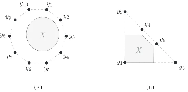
In brief, we consider a queueing network where the queue occupancy of thej’th queue
at time k is denoted by Qk(j) ∈ N, j = 1,2, . . . , n, and we gather these together into
vector Qk ∈ Nn. Time is slotted and at each time step k = 1,2, . . . we select action
yk ∈ Y ⊂ Nn, e.g. selecting j’th element xk(j) = 1 corresponds to transmitting one
packet from queuej and xk(j) = 0 to doing nothing. The connectivity between queues is
captured via matrix A ∈ {−1,0,1}n×n, whose j’th row has a −1 at the j’th entry, 1 at entries corresponding to queues from which packets are sent to, and 0 entries elsewhere.
The queue occupancy then updates according toQk+1= [Qk+Ayk+bk]+, where thej’th
element of vector bk ∈ Nn denotes the number of external packet arrivals to queue j at
time k. The objective is to stabilise all of the queues in the system while maximising a
concave utility U :Rn→R of the running average of the discrete actionsyi,i= 1, . . . , k.
In this chapter, we investigate the connections between max-weight approaches and
dual subgradient methods in convex optimisation, and show that strong connections do
indeed exist. We take as starting point the greedy primal-dual variant of max-weight
scheduling used by Stolyar [Sto05], which selects action yk ∈ arg maxy∈Y ∂U(xk)Ty −
βQTkAy withxk+1= (1−β)xk+βyk and 0< β <1 is a design parameter.
2.1. Preliminaries
Recall the following convexity properties.
Lemma2.1 (Lipschitz Continuity). Let ψ:M →R be a convex function and letX be a closed and bounded set contained in the relative interior of the domain M ⊆Rn. Then
ψis Lipschitz continuous on X i.e. there exists a constantνψ such that |ψ(x1)−ψ(x2)| ≤ νψkx1−x2k2 ∀x1, x2∈X.
Proof. See, for example, [RV74].
Lemma 2.2 (Bounded Distance). Let Y := {y1, . . . , y|Y|} be a finite set of points
from Rn. Then there exists constant y◦ such that kx1 −x2k2 ≤ y◦ for any two points x1, x2 ∈X:= conv(Y), where conv(Y) denotes the convex hull of Y.
Proof. Sincex1, x2 ∈X these can be written as the convex combination of points in
Y,i.e.
x1 =P|jY=1| θ(j)yj, x2 =P|jY=1| θ˜(j)yj
with θ,θ˜ 0, and kθk1 = kθ˜k1 = 1. Hence, kx1 −x2k2 = kP|jY=1|(θ(j) −θ˜(j))yjk2 ≤
P|Y|
j=1kθ(j)−θ˜(j)k2kyjk2 ≤2 maxy∈Y kyk2 :=y◦.
We also introduce the following definition:
Definition 2.1 (Bounded Curvature). Let ψ :M → R be a convex function defined on domain M ⊆Rn. We say ψ has bounded curvature on set X ⊂ M if for any points
x, x+δ∈X
ψ(x+δ)−ψ(x)≤∂ψ(x)Tδ+ρψkδk22 (2.1)
where ρψ ≥0 is a constant that does not depend on x or δ.
Bounded curvature will prove important in our analysis. The following lemma shows
that a necessary and sufficient condition for bounded curvature is that the subgradients
ofψ are Lipschitz continuous on setX.
Lemma 2.3 (Bounded Curvature). Let ψ :M → R, M ⊆Rn be a convex function. Thenψhas bounded curvature onX if and only if for allx, x+δ ∈Xthere exists a member
∂ψ(x) (respectively, ∂ψ(x+δ)) of the set of subdifferentials at pointx(respectively, x+δ)
such that
(∂ψ(x+δ)−∂ψ(x))T δ≤ρψkδk22
where ρψ does not depend onx or δ.
Proof. ⇒Suppose ψhas bounded curvature on X. From (2.1) it follows that
ψ(x+δ)−ψ(x)≤∂ψ(x)Tδ+ρψkδk22
and
ψ(x)−ψ(x+δ)≤ −∂ψ(x+δ)Tδ+ρψkδk22.
Adding the left-hand and right-hand sides of these inequalities yields 0≤(∂ψ(x)−∂ψ(x+
δ))Tδ+ 2ρ
ψkδk22 i.e.
⇐Suppose (∂ψ(x+δ)−∂ψ(x))T δ≤ρψkδk2 for all x, x+δ∈M. It follows that
∂ψ(x+δ)Tδ≤∂ψ(x)Tδ+ρψkδk22.
By the definition of the subgradient we have thatψ(x+δ)−ψ(x)≤∂ψ(x+δ)Tδ, and so
we obtain thatψ(x+δ)−ψ(x)≤∂ψ(x)Tδ+ρψkδk22.
2.2. Non-Convex Descent
We begin by considering the minimisation of convex functionF :Rn →R on convex setX := conv(Y), the convex hull of setY :={y1, . . . , y|Y|}consisting of a finite collection
of points fromRn (so X is a polytope). Our interest is in selecting a sequence of points {yk}, k = 1,2, . . . from set Y such that the running average xk+1 = (1−β)xk+βyk
minimisesF forksufficiently large andβ sufficiently small. Note that setY is non-convex
since it consists of a finite number of points, and by analogy with max-weight terminology
we will refer to it as theaction set.
Since X is the convex hull of action set Y, any point s∗ ∈ X minimising F can be written as convex combinations of points in Y i.e. s∗ = P|jY=1| θ∗(j)yj, θ∗(j) ∈ [0,1],
kθk1 = 1. Hence, we can always construct sequence{yk}by selecting points from setY in
proportion to theθ∗(j), j= 1, . . . ,|Y|—that is, bya posteriori time-sharing (a posteriori
in the sense that we need to find minimums∗ before we can construct sequence{yk}). Of
more interest, however, it turns out that when function F has bounded curvature then
sequences{yk} can be found without requiring knowledge ofs∗.
2.2.1. Non-Convex Direct Descent. The following two fundamental results are the key to establishing Theorem 2.1.
Lemma 2.4. Let Y := {y1, . . . , y|Y|} be a finite set of points from Rn and X :=
conv(Y). Then, for any point x ∈X and vector z ∈ Rn there exists a point y ∈ Y such that zT(y−x)≤0.
Proof. Since x ∈ X := conv(Y), x = P|jY=1| θ(j)yj with P|jY=1| θ(j) = 1 and θ(j) ∈
[0,1]. Hence,
zT(y−x) =
|Y| X
j=1
θ(j)zT(y−yj).
Selecty∈arg minw∈Y zTw. Then zTy ≤zTyj for all yj ∈Y and sozT(y−x)≤0.
Lemma2.5 (Non-Convex Descent). Let F(x) be a convex function and suppose points
curvature on X with curvature constant ρF. Then, there exists at least one y ∈Y such
that
F((1−β)x+βy)≤F(x)−γβǫ
withγ ∈(0,1) provided 0< β≤(1−γ) min{ǫ/(ρFy◦2),1}.
Proof. By convexity,
F(x) +∂F(x)T(z−x)≤F(z)≤F(x)−ǫ.
Hence,∂F(x)T(z−x)≤ −ǫ. Now observe that fory∈Y we have (1−β)x+βy ∈X and
by the bounded curvature ofF onX
F((1−β)x+βy)
≤F(x) +β∂F(x)T(y−x) +ρFβ2ky−xk22
=F(x) +β∂F(x)T(z−x) +β∂F(x)T(y−z) +ρFβ2ky−xk22 ≤F(x)−βǫ+β∂F(x)T(y−z) +ρFβ2ky−xk22
By Lemma 2.4 we can selecty∈Y such that∂F(x)T(y−z)≤0. With this choice of y it
follows that
F((1−β)x+βy)≤F(x)−βǫ+ρFβ2ky−xk22 ≤F(x)−βǫ+ρFβ2y◦2
(2.2)
where (2.2) follows from Lemma 2.2, and the result now follows.
The following theorem formalises the above commentary, also generalising it to
se-quences of convex functions {Fk} rather than just a single function as this will prove
useful later.
Theorem 2.1 (Greedy Non-Convex Convergence). Let {Fk} be a sequence of convex
functions with uniformly bounded curvatureρF on setX:= conv(Y), action setY a finite
set of points fromRn. Let{xk}be a sequence of vectors satisfyingxk+1 = (1−β)xk+βyk
withx1∈X and
yk ∈arg min
y∈Y Fk((1−β)xk+βy), k= 1,2, . . .
(2.3)
Suppose parameter β is sufficiently small that
0<β ≤(1−γ) min{ǫ/(ρFy2◦),1}
with ǫ > 0, γ ∈ (0,1), y◦ := 2 maxy∈Y kyk2 and that functions Fk change sufficiently
slowly that
|Fk+1(x)−Fk(x)| ≤γ1γβǫ, ∀x∈X
withγ1∈(0,1/2). Then, there exists a ¯k∈Nsuch that for all k≥k¯ we have that
0≤Fk(xk+1)−Fk(s∗k)≤2ǫ
where s∗k∈arg minx∈XFk(x).
Proof. SinceFk has bounded curvature for anykit is continuous, and asX is closed
and bounded we have by the Weierstrass theorem (e.g. see Proposition 2.1.1 in [BNO03])
that minx∈XFk(x) is finite. We now proceed considering two cases:
Case (i): Fk(xk)−Fk(s∗k)≥ǫ. By Lemma 2.5 there existsyk∈Y such that
Fk((1−β)xk+βyk)−Fk(xk) =Fk(xk+1)−Fk(xk)≤ −γβǫ.
Further, sinceFk+1(xk+1)−Fk(xk+1)≤γ1γβǫ andFk(xk)−Fk+1(xk)≤γ1γβǫit follows
Fk+1(xk+1)−Fk+1(xk)≤2γ1γβǫ−γβǫ <0. (2.5)
That is, Fk and Fk+1 decrease monotonically whenFk(xk)−Fk(s∗k)≥ǫ.
Case (ii): Fk(xk)−Fk(s∗k)< ǫ. It follows thatFk(xk)< Fk(s∗k) +ǫ. SinceFk is convex
and has bounded curvature,
Fk(xk+1)≤Fk(xk) +β∂Fk(xk)T(yk−xk) +β2ρFy2◦
≤Fk(s∗k) +ǫ+β∂Fk(xk)T(yk−xk) +β2ρFy2◦.
The final term holds uniformly for allyk ∈Y and since we selectyk to minimiseFk(xk+1) by Lemma 2.4 we therefore haveFk(xk+1)≤Fk(s∗k) +ǫ+β2ρFy◦2. Using the stated choice
ofβ and the fact that Fk+1(xk+1)−γ1γβǫ≤Fk(xk+1) yields
Fk+1(xk+1)−Fk(sk∗)≤γ1γβǫ+ǫ+β(1−γ)ǫ. (2.6)
Finally, since Fk(s∗k)≤Fk(sk∗+1)≤Fk+1(s∗k+1) +γ1γβǫ we obtain
Fk+1(xk+1)−Fk+1(s∗k+1)≤2γ1γβǫ+ǫ+β(1−γ)ǫ ≤2ǫ.
We therefore have that Fk+1(xk) is strictly decreasing when Fk(xk) −Fk(s∗k) ≥ ǫ
and otherwise uniformly upper bounded by 2ǫ. It follows that for all k sufficiently large
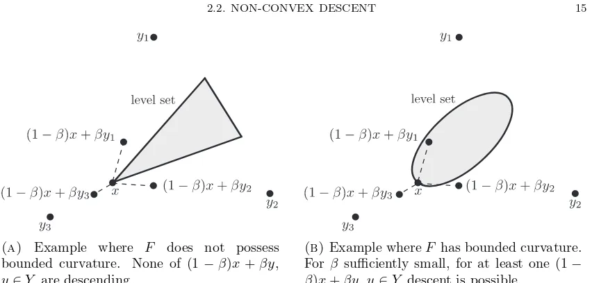
(a) Example where F does not possess bounded curvature. None of (1−β)x+βy,
y∈Y are descending.
(b)Example whereF has bounded curvature. For β sufficiently small, for at least one (1−
[image:20.595.102.528.77.281.2]β)x+βy,y∈Y descent is possible.
Figure 2.2.1. Illustrating how bounded curvature allows monotonic descent. Set
Y consists of the marked points y1, y2, y3. Level set {F(z) ≤F(x) :z ∈X} is
indicated by the shaded areas. The possible choices of (1−β)x+βy, y ∈Y are indicated.
Observe that in Theorem 2.1 we select ykby solving non-convex optimisation (2.3) at
each time step. This optimisation is one step ahead, or greedy, in nature and does not look
ahead to future values of the sequence or require knowledge of optimas∗k. Of course, such an approach is mainly of interest when non-convex optimisation (2.3) can be efficiently
solved,e.g. when action setY is small or the optimisation separable.
Observe also that Theorem 2.1 relies upon the bounded curvature of the sequence
of functions Fk. A smoothness assumption of this sort seems essential, since when it
does not hold it is easy to construct examples where Theorem 2.1 does not hold. Such
an example is illustrated schematically in Figure 2.2.1a. The shaded region in Figure
2.2.1a indicates the level set {F(z) ≤ F(x) : z ∈ X}. The level set is convex, but
the boundary is non-smooth and contains “kinks”. We can select points from the set
{(1−β)x+βy : y ∈ Y = {y1, y2, y3}}. This set of points is indicated in Figure 2.2.1a and it can be seen that every point lies outside the level set. Hence, we must have
F((1−β)x+βy) > F(x), and upon iterating we will end up with a diverging sequence.
Note that in this example changing the step size β does not resolve the issue. Bounded
curvature ensures that the boundary of the level sets is smooth, and this ensures that for
sufficiently smallβ there exists a convex combination of x with a point y ∈Y such that
F((1−β)x+βy)< F(x) and so the solution to optimisation (2.3) improves our objective,
Theorem 2.1 is stated in a fairly general manner since this will be needed for our later
analysis. An immediate corollary to Theorem 2.1 is the following convergence result for
unconstrained optimisation.
Corollary 2.1 (Unconstrained Optimisation). Consider the following sequence of
non-convex optimisations {Pk}:
yk ∈arg min
y∈Yf((1−β)xk+βy)
xk+1= (1−β)xk+βyk
with x1 ∈ X := conv(Y), action set Y ⊂ Rn finite. Then 0 ≤ f(xk) −f⋆ ≤ 2ǫ for
all k sufficiently large, where f⋆ = minx∈Xf(x), provided f has bounded curvature with
curvature constant ρF and 0 < β ≤ (1 −γ) min{ǫ/(ρFy2◦),1} with γ ∈ (0,1), ǫ > 0, y◦:= 2 maxy∈Y kyk2.
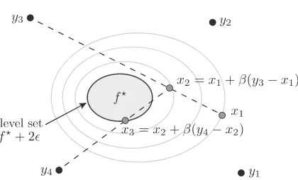
Figure 2.2.2 illustrates Corollary 2.1 schematically inR2. The sequence of non-convex optimisations descends in two iterations f(x1) > f(x2) > f(x3) (using points y3 and y4
respectively) andf(xk)−f⋆≤2ǫfork >3 (not shown in Figure 2.2.2).
Note that the curvature constantρF of functionf need not be known, an upper bound
being sufficient to selectβ. Next we present two brief examples that are affected differently
by constant ρF.
Example 2.1 (Linear Objective). Suppose f(x) :=ATx withA ∈Rn. The objective function is linear and so has curvature constant ρF = 0. It can be seen from (2.4) that
we can choose β independently of parameter ǫ. Hence, for any β ∈ (0,1) we have that
f(xk+1)< f(xk)for allk, and since we could always “choose” a smaller ǫ(becauseβ does not depend on it) we must have that f(xk)→f⋆.
Example 2.2 (Quadratic Objective). Suppose f(x) := 12xTAx where A ∈ Rn×n is
symmetric and positive definite. Then ρF =λmax(A) >0 and in contrast to Example 2.1
the bound (2.4) on parameter β now depends on ǫ. Further, the convergence is into the
ball f(xk)−f⋆ ≤2ǫ for k≥¯k and finite ¯k.
2.2.2. Non-Convex Frank-Wolfe-like Descent. It is important to note that other convergent non-convex updates are also possible. For example:
Theorem2.2 (Greedy Non-Convex FW Convergence). Consider the setup in Theorem
2.1, but with modified update
yk∈arg min
y∈Y ∂Fk(xk)
Ty, k= 1,2, . . .
Figure 2.2.2. Illustrating unconstrained convergence in R2. The sequence of non-convex optimisations converges with k = 2. The function average decreases monotonically and then remains in level setf(xk)≤f⋆+ 2ǫfork≥3.
Then, there exists ak¯∈N such that for all k≥¯k we have that
0≤Fk(xk+1)−Fk(s∗k)≤2ǫ
where s∗k∈arg minx∈XFk(x).
Proof. Firstly, we make the following observations,
arg min
x∈XFk(xk) +∂Fk(xk)
T(x−x k)
(a)
= arg min
x∈X∂Fk(xk) Tx
(b)
⊇ arg min
y∈Y ∂Fk(xk) Ty
where equality (a) follows by dropping terms not involvingxand (b) from the observation
that we have a linear program (the objective is linear and setX is a polytope, so defined
by linear constraints) and so the optimum lies at an extreme point of set X i.e. in set Y.
We also have that
Fk(xk) +∂Fk(xk)T(yk−xk)
(a)
≤ Fk(xk) +∂Fk(xk)T(s∗k−xk)
(b)
≤ Fk(s∗k)≤Fk(xk)
wheres∗k∈arg minx∈XFk(x), inequality (a) follows from the minimality ofyk inX noted
above and (b) from the convexity of Fk. It follows that ∂Fk(xk)T(yk−xk)≤ −(Fk(xk)−
Fk(s∗k)) ≤ 0. We have two cases to consider. Case (i): Fk(xk)−Fk(s∗k) ≥ ǫ. By the
bounded curvature of Fk,
Fk(xk+1)≤Fk(xk) +β∂Fk(xk)T(yk−xk) +ρFβ2y2◦
Hence,
Fk+1(xk+1)≤Fk(xk+1) +|Fk+1(xk+1)−Fk(xk+1)| ≤Fk(xk)−γβǫ+γ1γβǫ,
and sinceFk(xk)≤Fk+1(xk) +γ1γβǫ we have thatFk+1(xk+1)−Fk(xk+1)<0. Case (ii): Fk(xk)−Fk(s∗k)< ǫ. Then
Fk(xk+1)≤Fk(xk) +β∂Fk(xk)T(yk−xk) +ρFβ2y2◦
≤Fk(s∗k) +ǫ+βǫ,
and similar to the proof of Theorem 2.1 we obtain thatFk+1(xk+1)−Fk+1(s∗k+1)≤2ǫ. We therefore have that Fk(xk) is strictly decreasing when Fk(xk)−Fk(s∗k)≥ǫand otherwise
uniformly upper bounded by 2ǫ. Thus for ksufficiently large Fk(xk+1)−Fk(s∗k)≤2ǫ.
The intuition behind the update in Theorem 2.2 is that at each step we locally
approx-imateFk(xk+1) by linear function Fk(xk) +∂Fk(xk)T(xk+1−xk) and then minimise this
linear function. SinceFkis convex, this linear function is in fact the supporting hyperplane
to Fk at point xk, and so can be expected to allow us to find a descent direction. Similar
intuition also underlies classical Frank-Wolfe algorithms for convex optimisation [FW56]
on a polytope, and Theorem 2.2 extends this class of algorithms to make use of non-convex
update (2.7) and a fixed step size (rather than the classical approach of selecting the step
size by line search).
Note that when the function is linear Fk(x) =ckTx,ck∈Rn, then
arg min
y∈Y Fk((1−β)x+βy) = arg miny∈Y c T ky
(2.8)
and
arg min
y∈Y ∂Fk(xk)
Ty= arg min y∈Y c
T ky.
(2.9)
That is, updates (2.3) and (2.7) are identical. Note also that
arg min
y∈Y ∂Fk(xk)
Ty ⊆arg min
x∈X∂Fk(xk) Tx.
(2.10)
This is because the RHS of (2.10) is a linear programme (the objective is linear and set
X is a polytope, so defined by linear constraints) and so the optimum set is either (i)
an extreme point of X and so a member of set Y, or (ii) a face of polytope X with the
extreme points of the face belonging to setY. Hence, while update (2.7) is non-convex it
2.3. Constrained Convex Optimisation
We now extend consideration to the constrained convex optimisationP:
minimise
x∈X f(x)
subject to g(x)0 (2.11)
where g(x) := [g1, . . . , gm]T and f, gj :Rn → R, j = 1, . . . , m are convex functions with
bounded curvature with, respectively, curvature constantsρF andρgj. As before, action set Y consists of a finite set of points inRnandX:= conv(Y). LetX0 :={x∈X |g(x)0} denote the set of feasible points, which we will assume has non-empty relative interior
(i.e. a Slater point exists). Let X⋆ := arg minx∈X0f(x) ⊆X0 be the set of optima and f⋆:=f(x⋆),x⋆ ∈X⋆.
In the next sections we introduce a generalised dual subgradient approach for finding
approximate solutions to optimisationP which, as we will see, includes the classical convex
dual subgradient method as a special case.
2.3.1. Lagrangian Penalty. As in classical convex optimisation we define Lagrangian L(x, λ) := f(x) +λTg(x) where λ= [λ(1), . . . , λ(m)]T with λ(j) ≥0,j = 1, . . . , m. Since
setX0 has non-empty relative interior, the Slater condition is satisfied and strong duality
holds. That is, there is zero duality gap and so the solution of the dual problemD:
maximise
λ0 h(λ) := minx∈XL(x, λ)
and primal problemP coincide. Therefore, we have that
min
x∈Xmaxλ0 L(x, λ) = maxλ0 minx∈XL(x, λ) =h(λ ⋆) =f⋆
whereλ⋆:= arg max
λ0h(λ).
2.3.1.1. Lagrangian Bounded Curvature. As already noted, bounded curvature plays
a key role in ensuring convergence to an optimum when selecting from a discrete set of
actions. For any two pointsx, x+δ∈X we have that
L(x+δ, λ)≤L(x, λ) +∂xL(x, λ)Tδ+ρLkδk22,
where ρL = ρF +λTρg with ρg := [ρg1, . . . , ρgm]T. It can be seen that the curvature constantρLof the Lagrangian depends on the multiplierλ. Since setλ0 is unbounded,
it follows that the Lagrangian does not have bounded curvature on this set unless ρg =
0 (corresponding to the special case where the constraints are linear). Fortunately, by
has uniform bounded curvature with constant
¯
ρL=ρF +λ◦kρgk1.
For bounded curvature we only require constantλ◦ to be finite, but as we will see later in Lemmas 2.7 and 2.9 in general it should be chosen with some care.
2.3.2. Non-Convex Dual Subgradient Update. In this section we present a primal-dual-like approach in which we use discrete actions to obtain approximate
solu-tions to problemP. In particular, we construct a sequence{xk} of points in X such that
f(1kPki=1xi+1) is arbitrarily close tof⋆ forksufficiently large.
We start by introducing two lemmas, which will play a prominent role in later proofs.
Lemma 2.6 (Minimising Sequence of Lagrangians). Let {λk} be a sequence of vectors
in Rm+ such that λk λ◦1, λ◦ > 0 and kλk+1 −λkk2 ≤ γ1γβǫ/(mσc) with γ ∈ (0,1),
γ1 ∈ (0,1/2), β, ǫ > 0, σc := maxx∈Xkg(x)k∞. Consider optimisation problem P and
updates
yk∈arg min
y∈Y L((1−β)xk+βy, λk),
(2.12)
xk+1= (1−β)xk+βyk.
(2.13)
Then, for k sufficiently large (k≥k¯) we have that
L(xk+1, λk)−h(λk)≤L(xk+1, λk)−f⋆ ≤2ǫ
providedβis sufficiently small,i.e. 0<β≤(1−γ) min{ǫ/(¯ρLy◦2),1}wherey◦ := 2 maxy∈Y kyk2, ¯
ρL=ρF +λ◦kρgk1.
Proof. Observe that since
|L(x, λk+1)−L(x, λk)|=|(λk+1−λk)Tg(x)|
≤ kλk+1−λkk2kg(x)k2 ≤ kλk+1−λkk2mσc
≤γ1γβǫ
and L(·, λk) has uniformly bounded curvature by Theorem 2.1 we have that for k
suffi-ciently large (k≥¯k) then
where h(λ) := minx∈XL(x, λ). Further, since h(λ) ≤h(λ⋆) ≤f⋆ for all λ0 it follows
that
L(xk+1, λk)−f⋆≤2ǫ
fork≥¯k.
Lemma 2.7 (Lagrangian of Averages). Consider optimisation problem P and update
λk+1 = [λk+αg(xk+1)][0,λ
◦]
where α >0 and{xk} is a sequence of points from X such that L(xk+1, λk)−h(λk)≤2ǫ
for all k = 1,2, . . .. Let λ1(j) ∈ [0, λ◦] where λ◦ ≥λ⋆(j), j = 1, . . . , m, where λ⋆ ∈ Λ⋆ (the set of dual optima). Then,
|L(¯xk,λ¯k)−f⋆| ≤2ǫ+
α 2mσ
2
c +
mλ◦2 αk (2.14)
where x¯k := 1kPki=1xi+1,λ¯k:= 1kPki=1λi and σc := maxx∈Xkg(x)k∞.
Proof. Letθ∈Rm+ such thatθ(j)≤λ◦ for all j= 1, . . . , mand see that
kλk+1−θk22=k[λk+αg(xk+1)][0,λ
◦
]−θk2 2
≤ k[λk+αg(xk+1)]+−θk22 (2.15)
≤ kλk+αg(xk+1)−θk22
=kλk−θk22+ 2α(λk−θ)Tg(xk+1) +α2kg(xk+1)k22 ≤ kλk−θk22+ 2α(λk−θ)Tg(xk+1) +α2mσ2c,
(2.16)
where (2.15) follows since λ◦ ≥θ(j) and (2.16) from the fact that kg(x)k2
2 ≤mσc2 for all
x ∈ X. Applying the latter argument recursively for i = 1, . . . , k yields kλk+1−θk22 ≤ kλ1−θk22+ 2α
Pk
i=1(λi−θ)Tg(xi+1) +α2mσc2k. Rearranging terms, dividing by 2αk, and
using the fact thatkλk+1−θk22≥0 and kλ1−θk22 ≤2mλ◦2 we have
−mλ
◦2
αk −
α 2mσ
2
c ≤
1 k
k X
i=1
(λi−θ)Tg(xi+1) (2.17)
= 1 k
k X
i=1
L(xi+1, λi)−L(xi+1, θ). (2.18)
Next, see that by the definition of sequence {xk} we can write 1kPki=1L(xi+1, λi) ≤
1
k Pk
h. That is,
−mλ
◦2
αk −
α 2mσ
2
c −2ǫ≤h(¯λk)−
1 k
k X
i=1
L(xi+1, θ) (2.19)
By fixing θ to λ⋆ and ¯λk and using the fact that k1Pki=1L(xi+1,λ¯k) ≥ L(¯xk,λ¯k) for all
k= 1,2, . . . and k1Pki=1L(xi+1, λ⋆)≥f⋆ we have that
−mλ
◦2
αk −
α 2mσ
2
c −2ǫ≤h(¯λk)−f⋆ ≤0
(2.20)
and
−mλ
◦2
αk −
α 2mσ
2
c −2ǫ≤h(¯λk)−L(¯xk,λ¯k)≤0.
(2.21)
Multiplying (2.20) by−1 and combining it with (2.21) yields the result.
Note that by selecting α sufficiently small in Lemma 2.7 we can obtain a sequence
{λk} that changes sufficiently slowly so to satisfy the conditions of Lemma 2.6. Further,
by Lemma 2.6 we can construct a sequence of primal variables that satisfy the conditions
of Lemma 2.7 fork≥k¯ and it then follows that (2.14) is satisfied.
Lemma 2.7 requires that λ⋆(j) ≤ λ◦ for all j = 1, . . . , m, so it naturally arises the
question as to when λ⋆(j) (and so λ◦) is bounded. This is clarified in the next lemma,
which corresponds to Lemma 1 in [NO09a].
Lemma 2.8 (Bounded Multipliers). Let Qδ := {λ0 :h(λ) ≥h(λ⋆)−δ} with δ ≥0
and let the Slater condition hold, i.e. there exists a vector xˆ ∈ X such that g(ˆx) ≺ 0.
Then, for every λ∈Λδ we have that
kλk2 ≤ 1
υ(f(ˆx)−h(λ
⋆) +δ)
(2.22)
where υ:= minj∈{1,...,m}−gj(ˆx).
Proof. First of all recall that since the Slater condition holds we have strong duality,
i.e. h(λ⋆) =f⋆, andf⋆ is finite by Proposition 2.1.1. in [BNO03]. Now observe that when λ∈Λδ then
h(λ⋆)−δ ≤h(λ) = min
x∈XL(x, λ)≤f(ˆx) +λ Tg(ˆx),
and rearranging terms we obtain
−λTg(ˆx) =−
m X
j=1
Next, since λ 0 and−gj(ˆx) >0 for all j = 1, . . . , m, let υ:= minj∈{1,...,m}−gj(ˆx) and
see that υPmj=1λ(j) ≤f(ˆx)−h(λ⋆) +δ. Finally, dividing by υ and using the fact that
kλk2≤Pmj=1λ(j) the stated result follows.
From Lemma 2.8 we have that it is sufficient forX0to have non-empty relative interior
in order for Λδ to be a bounded subset inRm+, and since by definition λ⋆ ∈Λδ thenλ⋆ is
bounded. The bound obtained in Lemma 2.8 depends onh(λ⋆) =f⋆, which is usually not known. Nevertheless, we can obtain a looser bound if we use the fact that−h(λ⋆)≤ −h(λ) for all λ0. That is, for everyλ∈Λδ we have that
kλk2≤ 1
υ(f(¯x)−h(λ0) +δ),
whereλ0 is an arbitrary vector inRm+.
Hence, when the Slater condition is satisfied the upper and lower bounds in (2.14) are
finite and can be made arbitrarily small ask→ ∞by selecting the step sizeα sufficiently
small. Convergence of the average of the Lagrangians does not, of course, guarantee that
f(¯xk) →f⋆ unless we also have complementary slackness, i.e. (¯λk)Tg(¯xk)→ 0. Next we
present the following lemma, which is a generalisation of Lemma 3 in [NO09a].
Lemma 2.9 (Complementary Slackness and Feasibility). Let the Slater condition hold
and suppose {xk} is a sequence of points in X and{µk} a sequence of points inRm+ such
that
(i) L(xk+1, µk)−h(µk)≤2ǫfor all k;
(ii) |λk(j)−µk(j)| ≤ασ0, j= 1, . . . , m
where λk+1 = [λk+αg(xk+1)]+, ǫ ≥0, α >0, σ0 ≥ 0. Suppose also that λ1(j) ∈[0, λ◦]
with
λ◦≥ υ3(f(ˆx)−h(λ⋆) +δ) +αmσc
where δ := α(mσ2
c/2 +m2σ0σc) + 2ǫ, σc := maxx∈Xkg(x)k∞, xˆ a Slater vector and υ:= minj∈{1,...,m}−gj(ˆx). Then, λk(j)≤λ◦ for allk= 1,2, . . .,
−mλ
◦2 2αk −
α 2mσ
2
c ≤(¯λk)Tg(¯xk)≤
mλ◦2 αk (2.23)
and
gj(¯xk)≤
λ◦ αk (2.24)
Proof. We start by showing that updates [λk+αg(xk+1)]+ and [λk+αg(xk+1)][0,λ
◦
]
are interchangeable whenL(xk+1, µk) is uniformly close toh(µk). First of all see that
kλk+1−λ⋆k22 =k[λk+αg(xk+1)]+−λ⋆k22 ≤ kλk+αg(xk+1)−λ⋆k22
=kλk−λ⋆k22+α2kg(xk+1)k22+ 2α(λk−λ⋆)Tg(xk+1) ≤ kλk−λ⋆k22+α2mσ2c + 2α(λk−λ⋆)Tg(xk+1).
Now observe that sincekλk−µkk2 ≤ kλk−µkk1 ≤αmσ0 we can write
(λk−λ⋆)Tg(xk+1) = (µk−λ⋆)Tg(xk+1) + (λk−µk)Tg(xk+1) ≤(µk−λ⋆)Tg(xk+1) +kλk−µkk2kg(xk+1)k2 ≤(µk−λ⋆)Tg(xk+1) +αm2σ0σc
=L(xk+1, µk)−L(xk+1, λ⋆) +αm2σ0σc.
Furthermore, sinceL(xk+1, µk)≤h(µk) + 2ǫand −L(xk+1, λ⋆)≤ −h(λ⋆) it follows that
kλk+1−λ⋆k22− kλk−λ⋆k22
≤α2(mσc2+ 2m2σ0σc) + 2α(h(µk) + 2ǫ−h(λ⋆)).
(2.25)
Now let Λδ:={λ0 :h(λ)≥h(λ⋆)−δ} and consider two cases. Case (i) (µk ∈/ Qδ).
Then h(µk)−h(λ⋆)<−δ and from (2.25) we have thatkλk+1−λ⋆k22 <kλk−λ⋆k22,i.e.
kλk+1−λ⋆k2− kλk−λ⋆k2 <0
and soλkconverges to a ball around λ⋆ whenµk∈Λδ. Case (ii) (µk∈Qδ). Observe that
kλk+1−λ⋆k2 =k[λk+αg(xk+1)]+−λ⋆k2 ≤ kλk+αg(xk+1)−λ⋆k2 ≤ kλkk2+kλ⋆k2+αmσc.
Next recall that when the Slater condition holds by Lemma 2.8 we have for all λ ∈ Λδ
thenkλk2 ≤ 1υ(η+δ) whereη:=f(¯x)−h(λ⋆) and ¯x a Slater vector. Therefore,
kλk+1−λ⋆k2≤ 2
υ(η+δ) +αmσc. From both cases, it follows that if
kλ1−λ⋆k2≤ 2
thenkλk−λ⋆k2 ≤ υ2(η+δ) +αmσc for allk≥1. Using this observation and the fact that
kλ1−λ⋆k2 ≥ |kλ1k2− kλ⋆k2| ≥ kλ1k2− kλ⋆k2
we obtain that whenkλ1k2≤ υ3(η+δ) +αmσc thenkλkk2 ≤ 3υ(η+δ) +αmσc for allk≥1.
That is, if we chooseλ1(j)≤ 3υ(η+δ) +αmσc ≤λ◦ then λk(j)≤λ◦ for all j = 1, . . . , m,
k ≥ 1 and so updates [λk +g(xk+1)]+ and [λk +g(xk+1)][0,λ
◦]
are interchangeable as
claimed.
Now we proceed to prove the upper and lower bounds in (2.23). For the lower bound
see first that
kλk+1k22 =k[λk+αg(xk+1)]+k22 ≤ kλk+αg(xk+1)k22
=kλkk22+α2kg(xk+1)k22+ 2αλTkg(xk+1) ≤ kλkk22+α2mσc2+ 2αλTkg(xk+1)
Rearranging terms and applying the latter bound recursively fori= 1, . . . , k yields
2α
k X
i=1
λTi g(xi+1)≥ kλk+1k22− kλ1k22−α2mσc2k≥ −kλ1k22−α2mσc2k.
The bound does not depend on sequence{xk}, hence, it holds for any sequence of points
inX. Fixingxi+1 to ¯xk for all i= 1, . . . , k we can write
2α
k X
i=1
λTi g(¯xk) = 2αk(¯λk)Tg(¯xk)
Dividing by 2αk and using the fact that kλ1k22 ≤mλ◦2 yields
−mλ
◦
2αk − α 2mσ
2
c ≤(¯λk)Tg(¯xk).
For the upper bound see that λk+1 = [λk+αg(xk+1)]+ λk+αg(xk+1) and so we can write
α
k X
i=1
g(xi+1)
k X
i=1
(λi+1−λi) =λk+1−λ1 λk+1.
Next, by the convexity of g we have that
1 k
k X
i=1
and so it follows that g(¯xk) λk+1/(αk). Multiplying the last equation by ¯λk and using
the fact that 0 λk+1 λ◦1 and 0 λ¯k λ◦1 yields the upper bound. Finally, the
constraint violation bound (2.24) follows from the fact that g(¯xk)λ◦2/(αk)1.
Lemma 2.9 is expressed in a general form whereµmay be any suitable approximation
to the usual Lagrange multiplier. Evidently, the lemma also applies in the special case
whereλk =µkin which caseσ0 = 0. Note from the lemma as well that the running average ¯
xk is asymptotically attracted to the feasible region as kincreases, i.e. limk→∞g(¯xk)0
We are now in a position to present one of our main results:
Theorem2.3 (Constrained Optimisation). Consider constrained convex optimisation P and the associated sequence of non-convex optimisations {P˜k}:
yk∈arg min
y∈Y L((1−β)xk+βy, µk)
(2.26)
xk+1= (1−β)xk+βyk
(2.27)
λk+1= [λk+αg(xk+1)][0,λ
◦
] (2.28)
Let the Slater condition hold and suppose that |λk(j)−µk(j)| ≤ασ0 for all j= 1, . . . , m, k ≥ 1 with σ0 ≥ 0. Further, suppose parameters α and β are selected sufficiently small
that
0< α≤γ1γβǫ/(m2(σc2+ 2σ0σc))
(2.29)
0< β≤(1−γ) min{ǫ/(¯ρLy◦2),1}
(2.30)
with ǫ >0, γ ∈(0,1), γ1 ∈(0,1/2), y◦ := 2 maxy∈Y kyk2, ρ¯L =ρF +λ◦kρgk1 and λ◦ as
given in Lemma 2.9. Then, for k sufficiently large (k≥¯k) the sequence of solutions {xk}
to sequence of optimisations {P˜k} satisfies:
−2mλ
◦2
αk −α(mσ 2
c/2 +m2σ0σc)−2ǫ
≤f(¯xk)−f⋆≤2ǫ+α(mσc2+m2σ0σc) +
3mλ◦2 2αk (2.31)
where x¯k := 1k P¯k+k
i=¯k xi+1, µ¯k:=
1
k P¯k+k
Proof. First of all observe that sinceλk+1(j) = [λk(j) +αgj(xk+1)][0,λ
◦
]we have that
|λk+1(j)−λk(j)| ≤ασc for all k. Further, since |λk(j)−µk(j)| ≤ασ0 then
|µk+1(j)−µk(j)|=|µk+1(j)−µk(j) +λk+1(j)−λk+1(j) +λk(j)−λk(j)|
≤ |µk+1(j)−λk+1(j)|+|λk+1(j)−λk(j)|+|λk(j)−µk(j)|
≤α(2σ0+σc).
That is,
kµk+1−µkk2 ≤αm(2σ0+σc) k= 1,2, . . .
(2.32)
Next, observe that sinceL(·, λk) has uniform bounded curvature and
|L(x, µk+1)−L(x, µk)| ≤ kµk+1−µkk2kg(xk+1)k2 ≤ kµk+1−µkk2mσc
≤αm2(2σ0σc+σc2)
≤γ1γβǫ,
it follows by Lemma 2.6 that forksufficiently large (k≥k¯) thenL(xk+1, µk)−h(µk)≤2ǫ
and therefore by Lemma 2.7
−mλ
◦2
αk −
α 2mσ
2
c −2ǫ≤L(¯xk,µ¯k)−f⋆≤2ǫ+
α 2mσ
2
c +
mλ◦2 αk .
Next, see that since
|L(¯xk,λ¯k)−L(¯xk,µ¯k)|= (¯λk−µ¯k)Tg(¯xk)
≤ kλ¯k−µ¯kk2kg(¯xk)k2 ≤αm2σ0σc
we have that
−mλ
◦2
αk −α(mσ 2
c/2 +m2σ0σc)−2ǫ
≤L(¯xk,λ¯k)−f⋆ ≤2ǫ+α(mσ2c/2 +m2σ0σc) +
mλ◦2 αk .
Finally, by using the complementary slackness bound of Lemma 2.9 the stated result
follows.
Theorem 2.3 says that by selecting step sizeαand smoothing parameterβ sufficiently
small then the average of the solutions to the sequence of non-convex optimisations{P˜k}
2.3.2.1. Alternative Update. Note that, by replacing use of Theorem 2.1 by Theorem
2.2 in the proof, we can replace update (2.26) by its non-convex Frank-Wolfe alternative,
yk∈arg min
y∈Y ∂xL(xk, µk) Ty
(2.33)
= arg min
y∈Y (∂f(xk) +µ T
k∂g(xk))Ty.
That is, we have:
Corollary2.2 (Constrained Optimisation Using Frank-Wolfe Update). Consider the
setup in Theorem 2.3 but with update (2.26) replaced by (2.33). Then, there exists a finite ¯
k such that the bound given in (2.31) holds.
2.3.3. Generalised Update. LetX′ ⊆conv(Y) be any subset of the convex hull of action setY, including the empty set. Since
min
y∈X′∪Y L((1−β)xk+βy, µk)≤miny∈Y L((1−β)xk+βy, µk), we can immediately generalise update (2.26) to
yk∈arg min y∈X′∪Y
L((1−β)xk+βy, µk)
(2.34)
and Theorem 2.3 will continue to apply. Selecting X′ equal to the empty set we recover (2.26) as a special case. Selecting X′ = conv(Y) we recover the classical convex dual
subgradient update as a special case. Update (2.34) therefore naturally generalises both
the classical convex dual subgradient update and non-convex update (2.26). Hence, we
have the following corollary.
Corollary 2.3 (Constrained Optimisation Using Unified Update). Consider the
setup in Theorem 2.3 but with update (2.26) replaced by (2.34). Then, there exists a
finite k¯ such that the bound given in (2.31) holds.
2.4. Using Queues as Approximate Multipliers
In Theorem 2.3 the only requirement on the sequence of approximate multipliers{µk}
is that it remains close to the sequence of Lagrange multipliers{λk} generated by a dual
subgradient update in the sense that |λk(j)−µk(j)| ≤ ασ0 for all k. In this section we consider the special case where sequence{µk}additionally satisfies the following,
µk+1 = [µk+ ˜δk][0,λ
◦
] (2.35)
We begin by recalling the following lemma, which is a direct result of [Mey08,
Propo-sition 3.1.2].
Lemma 2.10. Consider sequences {λk}, {µk} in R given by updates λk+1 = [λk +
δk][0,λ
◦]
andµk+1 = [µk+ ˜δk][0,λ
◦]
where δ,δ˜∈R. Suppose λ1=µ1 and |Pki=1δi−δ˜i| ≤ǫ
for allk. Then, for all k we have that |λk−µk| ≤2ǫ.
Proof. First of all observe that |λk+1−µk+1| = |[λk+δk][0,λ
◦]
−[µk+ ˜δk][0,λ
◦] | ≤ |[λk+δk][0,λ
◦
]−[µ
k+ ˜δk]+|=|[µk+ ˜δk]+−[λk+δk][0,λ
◦
]| ≤ |[µ
k+ ˜δk]+−[λk+δk]+|.We
now proceed to bound the RHS of the last equation. Let ∆k := −min(λk+δk,0), i.e.
λk+1 =λk+δk+ ∆k so that we can write
λk+1=λ1+
k X
i=1
(δi+ ∆i)
Note that when λk+1 > 0 then ∆k = 0, and that when λk+1 = 0 then Pki=1∆i = −λ1 −Pki=1δi. Next, note that since ∆k is nonnegative for all k by construction we
have that Pki=1∆i is non-decreasing in k. Using the latter observation it follows that Pk
i=1∆i= [−λ1−min1≤j≤kPji=1δi]+ and therefore
λk+1 =
k X
i=1
δi+ max{Θk, λ1}
where Θk:=−min1≤j≤kPji=1δi. Now, let ˜Θk:=−min1≤j≤kPji=1δ˜i and see that
|λk+1−µk+1|=
k X i=1
δi+ max{Θk, λ1} − k X
i=1 ˜
δi−max{Θ˜k, λ1} ≤ k X i=1 δi−˜δi
+
max{Θk, λ1} −max{Θ˜k, λ1}
(a) ≤ k X i=1 δi−δ˜i
+
Θ˜k−Θk = k X i=1 δi−˜δi
+ min 1≤j≤k
j X
i=1 ˜
δi− min
1≤j≤k j X i=1 δi = k X i=1 δi−˜δi
+ max 1≤j≤k
j X
i=1
−˜δi− max
1≤j≤k j X
i=1 −δi
≤ k X i=1 δi−˜δi
+ max 1≤j≤k
j X i=1 δi−
j X i=1 ˜ δi
where (a) follows easily from enumerating the four cases. Finally, since|Pki=1δi−˜δi| ≤
Applying Lemma 2.10 to our present context it follows that |λk(j)−µk(j)| ≤ασ0 for allk(and so Theorem 2.3 holds) for every sequence{δ˜k}such that|Pki=1αgj(xi)−δ˜i(j)| ≤
ασ0 for all k.
Of particular interest is the special case of optimisation P where the constraints are
linear. That is,gj(x) =a(j)x−b(j) where (a(j))T ∈Rnandb(j)∈R,j= 1, . . . , m.
Gath-ering vectors a(j) together as the rows of matrixA∈Rm×nand collecting additive terms b(j) into vector b∈Rm, the linear constraints can then be written as Axb. Therefore, the dual subgradient Lagrange multiplier update in the sequence of optimisations{P˜k} is
given by
λk+1= [λk+α(Axk+1−b)][0,λ
◦] (2.36)
withxk+1= (1−β)xk+βyk,yk∈Y. Now suppose that in (2.35) we select ˜δk=α(Ayk−bk)
where{bk} is a sequence of points inRm. Then,
µk+1= [µk+α(Ayk−bk)][0,λ
◦
] (2.37)
withµ1 =λ1.
Observe that in (2.37) we have replaced the continuous-valued quantity xk with the
discrete-valued quantity yk. We have also replaced the constant b with the time-varying
quantitybk. Further, letting Q:=µ/α then (2.37) can be rewritten equivalently as
Qk+1 = [Qk+Ayk−bk][0,λ
◦/α] (2.38)
which is a discrete queue length update with increment Ayk − bk. The approximate
multipliersµ are therefore scaled discrete queue occupancies.
Using Lemma 2.10 it follows immediately that Theorem 2.3 holds provided
|Pki=1a(j)(xi−yi) + (bi(j)−b(j))| ≤ασ0 (2.39)
Since updatexk+1= (1−β)xk+βykyields a running average of{yk}we might expect that
sequences {xk} and {yk} are always close and so uniform boundedness of|Pki=1(bi(j)−
b(j))|is sufficient to ensure that (2.39) is satisfied. This is indeed the case, as established
by the following theorem.
Theorem 2.4 (Queues as Approximate Multipliers). Consider updates (2.36) and
(2.37) where {yk} is an arbitrary sequence of points in Y, xk+1 = (1 −β)xk +βyk,

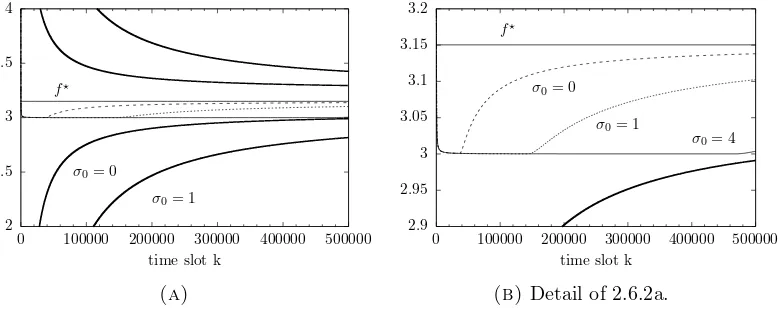
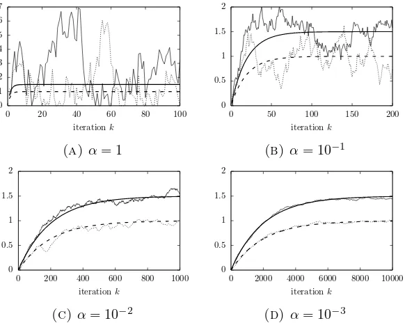
![Figure 2.6.3. Illustrating the violation of the bounds of Theorem 2.3 whenthicker lines indicate upper and lower bounds aroundµk(j) = [λk(j) + αeke−105][0,λ◦].Dashed line indicates f(¯xk), k¯ = 81, while f ⋆ (straight line).](https://thumb-us.123doks.com/thumbv2/123dok_us/173171.511227/42.595.216.417.95.247/illustrating-violation-theorem-whenthicker-indicate-arounduk-indicates-straight.webp)