Abstract— Standard roughness measurement procedures depend heavily on stylus instruments which have only limited flexibility in handling different parts. On the other hand, optical non-contact techniques are very interesting for 3D characterization of sensitive and complex engineering surfaces. In this study, a new approach is introduced to measure surface roughness in three dimensions by combining a light sectioning microscope and a computer vision system. This approach has the advantages of being non-contact, fast and cheep. A prototype version of a user interface program, currently named
SR3DVision, has been developed to manage three dimensional surface roughness measurements. A light sectioning microscope is used to view roughness profiles of the specimens to be measured and the vision system is used to capture images for successive profiles. This program has been totally developed in-house using Matlab™ software to analyze the captured images through four main modules: (Measurement controller, Profile or surface extraction, 2D roughness parameters calculation and 3D roughness parameters calculation). The system has been calibrated for metric units and verified using standard specimens. In addition, the system was used to measure various samples machined by different operations and the results were compared with a commercial software and a web-based surface metrology algorithm testing system. The accuracy of the system was verified and proved to be within ±4.8% compared with these systems.
Index Terms—3D surface roughness, Computer vision, Light sectioning.
I. INTRODUCTION
The development of new industries has led to a requirement for super-smooth surfaces and for the ability to measure surfaces of industrial parts accurately; therefore, the measurement of engineering surface roughness is becoming increasingly important. Many methods of measuring surface finish have been developed ranging from the simple touch comparator to sophisticated optical techniques [1]-[3]. Optical methodology [4]-[6] and computer vision systems [7]-[11] are the most common methods among the developed researches. Computer vision was implemented to measure surface roughness by many researchers [7]-[17]. Computer vision systems offers the advantages of the optical techniques, which tend to fulfill the need for quantitative characterization of surface topography without contact, whilst vision systems is considered relatively cheap and fast.
Unlike the stylus instruments, the optical techniques and computer vision systems have the advantages of being
Manuscript received January 11, 2010.
Ossama B. Abouelatta is with the Production Engineering and Mechanical Design Department, Faculty of Engineering, Mansoura University, 35516 Mansoura, Egypt (phone: +201-2737-9496; fax: +205-0224-4690; e-mail: [email protected]).
non-contact and are capable of measuring an area from the surface rather than a single line. Further the procedure is an in-process approach which is amenable for automation. Light sectioning methods are considered as an optical technique, which was initially proposed by Schmaltz [12] to get the roughness profile of surfaces. The use of light sectioning method combined with computer vision is suggested by many researchers [13]-[17].
In the recent past, higher levels of automation in the shop floor has focused the attention on the application of fast, reliable and cost effective procedures for evaluating surfaces of medium finished parts. Kiran et al. [13] covered in brief few finish assessment methods of medium rough surfaces using a standard vision system in order to achieve quick estimation of the finish of medium rough surfaces. A design of an optical instrument for 2D surface roughness measurement was demonstrated by Shou-Bin and Hui-Fen [14]. Based on these principles, a commercial optical instrument has been developed whose measurement height is in the range of 0.4-120 µm. Light sectioning of an object surface uses the line deformation imaged to compute the object profile was used by Lewandowaki and Desjardins [15]. A 2D surface roughness measurement system was designed with a light-sectioning microscope and the corresponding software was developed by Shou-Bin and Hui-Fen [16]. Their experimental results showed a feasible method for surface roughness measurement. In a previous work [17], the author introduced a system to measure two dimensional surface roughness by combining a light sectioning microscope and a computer vision system. The system was used to measure machined samples and the results were compared with the measurements of a stylus instrument.
The aim of this work is to introduce a new non-contact system for automatic three dimensional measurement of surface roughness by utilizing a light sectioning microscope and a computer vision system. Consequently, amplitude roughness parameters in three dimensions as well as most of the two dimension roughness parameters can be calculated by the introduced system.
II. EXPERIMENTAL SETUP
The introduced system consists of two major parts, hardware and software. A photograph of the system is shown in Fig. 1. The hardware consists of four items: personal computer (PC), a light sectioning microscope, a vision system and a precision table of Nikon Measurescope-10 derived by a stepper motor and its controller. The PC is an IBM-compatible personal computer with Pentium processor
3D Surface Roughness Measurement Using a
Light Sectioning Vision System
and Windows operating system. The light sectioning microscope is supplied with a suitable set of magnification lenses to produce magnified roughness profile
under investigation. The vision system consists of a JVC color video camera (CCD) and an ELF-VGA frame grabber provided with capturing software to capture images
[image:2.612.73.299.206.391.2]by the CCD camera. The CCD camera is fixed on the eyepiece of the light sectioning microscope using a special holder designed to provide an accurate alignment between the camera and the image reflected by the microscope frame grabber is fitted inside the PC and connected to the CCD camera. It is used to digitize the analogue image, produced by the CCD camera, into 760×570 pixels with 16 bits of color.
Fig. 1. Photograph of the introduced system. 1. Stepper motor. 7. Light section 2. Coupling. 8. Precision X-Y 3. Stepper motor controller. 9. Display counter. 4. CCD camera. 10. Power supply. 5. CCD camera holder. 11. Capturing s 6. Standard specimen. 12. Personal computer.
A specially developed program, named SR3DVision
been fully developed in-house using Matlab™ software and the provided image processing toolbox, to analyze the captured images. The SR3DVision program consists of four modules with a graphical user interface
[image:2.612.314.543.263.410.2]Measurement controller, profile or surface extraction, 2D roughness parameters calculation, and 3D roughness parameters calculation. All modules can be executed from main interface, Fig. 2.
Fig. 2. Main interface of SR3DVision program.
The first module (MeasControl) is used to control the measuring process via stepper motor and its controller After starting measurements, the x-y table is
11 10 9 7 6 5 4
1 2 3 8
and Windows operating system. The light sectioning microscope is supplied with a suitable set of magnification lenses to produce magnified roughness profiles for surfaces . The vision system consists of a JVC VGA frame grabber provided with capturing software to capture images acquired by the CCD camera. The CCD camera is fixed on the eyepiece of the light sectioning microscope using a special lignment between by the microscope. The frame grabber is fitted inside the PC and connected to the CD camera. It is used to digitize the analogue image, 570 pixels with 16
ection microscope. Y table. Display counter.
upply. software. omputer.
SR3DVision, has
using Matlab™ software and the provided image processing toolbox, to analyze the program consists of four modules with a graphical user interface, which are: Measurement controller, profile or surface extraction, 2D 3D roughness All modules can be executed from the
program.
is used to control the measuring process via stepper motor and its controller [18]. table is automatically
moved forward by 20 µ m to eliminate backlash from the driving system. Next, the user is prompted
name, number of traces (NTraces) and the sampling interval
∆y. These processes repeated Ntraces
Ntraces images.
The second module (ProfileExtract
extract the x-z coordinates of the roughness profiles from the captured images by performing various image processing and computer vision algorithms. Through this module captured image is opened and analyzed
roughness profile, then the x-z coordin
profile is saved to an ".SDF" file for further use by
SR3DVision program or other commercial software.
other hand, this module can be used to extract the coordinates of the successive profiles from the captured images. The x-z coordinates of the extracted profiles are saved to an ".SDF" file for further use by the
program or other commercial software.
Fig. 3. Profile extraction module (ProfileExtract
The third module (RP2DCalc), Fig. 4, the 2D roughness parameters [19]-[2
produced for each image by the second module
this module is used to view the 2D surface roughness profile extracted from each image.
Fig. 4. Two dimensional surface roughness parameters calculation module (RP2DCalc).
The fourth module (RP3DCalc), Fig. the 3D roughness parameters [21]
produced for all images by the second module. In addition, this module is used to view the 3D surface topography extracted from all captured images.
12
20 µ m to eliminate backlash from the prompted to enter data file and the sampling interval
Ntraces times to produce a
ProfileExtract), Fig. 3, is used to
coordinates of the roughness profiles from the captured images by performing various image processing and computer vision algorithms. Through this module, each analyzed to extract the 2D coordinates of the extracted file for further use by the or other commercial software. On the other hand, this module can be used to extract the x-z
coordinates of the successive profiles from the captured coordinates of the extracted profiles are file for further use by the SR3DVision
program or other commercial software.
ProfileExtract).
, Fig. 4, is used to calculate 20] from the SDF file produced for each image by the second module. In addition, surface roughness profile
roughness parameters
[image:2.612.313.543.503.646.2] [image:2.612.72.300.522.680.2]Fig. 5. Three dimensional surface roughness parameters calculation module (RP3DCalc).
III. PROCEDURES OF WORK
To calculate the 3D surface roughness parameters and visualize the 3D surface topography by the introduced system, the specimen to be measured is positioned on the table of the light sectioning microscope under the projected light. The focus is adjusted until the roughness profile appears clear on the screen of the capturing software (ELF-VGA). After selecting a suitable section, the capturing software is used to capture an image for the viewed profile and to save it to a bitmap image file (BMP). This step is repeated NTraces for 3D surface roughness measurement. Finally, the captured image is opened by the
program, then the processing algorithms are applied. The roughness parameters of the extracted profile can be calculated by selecting Calculate 2D or 3D parameters the main module, which display the second and third modules, as shown in Fig. 4 and Fig. 5, respectively.
IV. PROCESSING ALGORITHMS
Image processing and computer vision algorithms applied to analyze the captured images and to extract the roughness profiles as shown in Fig. 6. First, the algorithm check the depth of color in the opened image. If the image is colored, the software converts it to grey scale. Then, a global threshold is calculated to convert the grey scale image into a binary image (Black and white image). The upper and lower profiles are traced by locating upper and lower boundaries of the binary image. Finally, a calibration factor is applied extracted profiles in order to calculate the actual coordinates (See Section V). An SDF file is second and third modules for later use to calculate roughness parameters.
V. SYSTEM CALIBRATION
The system has been calibrated for light sectioning microscope lens in both x-direction (horizontal resolution) and z-direction (vertical resolution). A standard specimen produced by American Optical Company–Buffalo, was used to calibrate the system for horizontal resolution. The specimen has 2 mm scale divided into units of 0.01 mm. A Light section microscope lens was used to capture an ima for the scale of the standard specimen and the number of divisions was counted for each image to calculate the corresponding field of view as shown in Table I.
. Three dimensional surface roughness parameters
surface roughness parameters and to by the introduced system, the specimen to be measured is positioned on the table of the light sectioning microscope under the projected light. The focus is adjusted until the roughness profile on the screen of the capturing software section, the capturing software is used to capture an image for the viewed profiles save it to a bitmap image file (BMP). This step is ghness measurement. Finally, the captured image is opened by the SR3DVision
program, then the processing algorithms are applied. The roughness parameters of the extracted profile can be calculated by selecting Calculate 2D or 3D parameters from , which display the second and third
, respectively.
ROCESSING ALGORITHMS
Image processing and computer vision algorithms are applied to analyze the captured images and to extract the . First, the algorithms check the depth of color in the opened image. If the image is colored, the software converts it to grey scale. Then, a global threshold is calculated to convert the grey scale image into a ge). The upper and lower traced by locating upper and lower boundaries of the binary image. Finally, a calibration factor is applied to the to calculate the actual x and z
created by the to calculate surface
[image:3.612.344.505.46.308.2]The system has been calibrated for light sectioning direction (horizontal resolution) resolution). A standard specimen Buffalo, was used to calibrate the system for horizontal resolution. The specimen has 2 mm scale divided into units of 0.01 mm. A Light section microscope lens was used to capture an image for the scale of the standard specimen and the number of divisions was counted for each image to calculate the corresponding field of view as shown in Table I.
Fig. 6. Flowchart of the image processing algorithm extract surface heights data from the light sectioning profiles
Because the implied vision system produces images sized to 760×570 pixels, the horizontal resolution for each lens was calculated by dividing the value of the field of view (in µm) by the width of the captured image (760 pixels). The horizontal resolution (H) for a lens of 13.9 mm focal length can be calculated as follows:
Horizontal Resolution (H)
= Field of view/Width of the captured image = 1000/760 = 1.31579 µm/pixel
On the other hand, another standard specimen has an arithmetic average roughness Ra = 2.97 µ m and peak to
valley height roughness parameter Rt =
calibrate the system for the vertical resolution. Fig. Table II show a sample roughness profile of the standard specimen (4 mm length) obtained by a Surftest SJ201 instrument connected to a personal computer. At least twenty images were captured for two standard specimens, then a two roughness profiles (upper and lower) were extracted by the
SR3DVision program. Because the captured profiles may not
be exactly horizontal, the least square method was applied to the extracted profiles to remove any inclination in the surface. The maximum peak to valley height was calculated (in pixels) for each profile, then the average value was taken. The vertical resolution (V) was calculated by dividing the actual value of Rt by the calculated average as follows:
Vertical Resolution (V)
= 10.95/Rt = 0.9343 µ m/pixel
Table I summarizes the horizontal resolution
vertical resolution of the system for a pair of light section microscope lens.
Convert color image to grayscale Colored
image? Start
Read Image
Convert grayscale image to black and white
Trace the boundaries
Extract lower and upper profiles For i=1:No. of images
End Add to data (η)
Save data as an *.SDF file Yes
No
image processing algorithm used to light sectioning profiles. Because the implied vision system produces images sized 570 pixels, the horizontal resolution for each lens was calculated by dividing the value of the field of view (in µm) by the width of the captured image (760 pixels). The for a lens of 13.9 mm focal length
Field of view/Width of the captured image = 1.31579 µm/pixel
standard specimen has an = 2.97 µ m and peak to = 11.72 µ m was used to calibrate the system for the vertical resolution. Fig. 7 and a sample roughness profile of the standard specimen (4 mm length) obtained by a Surftest SJ201-P connected to a personal computer. At least twenty mages were captured for two standard specimens, then a two roughness profiles (upper and lower) were extracted by the program. Because the captured profiles may not be exactly horizontal, the least square method was applied to iles to remove any inclination in the surface. The maximum peak to valley height was calculated (in pixels) for each profile, then the average value was taken. was calculated by dividing the
average as follows:
µ m/pixel
Table I summarizes the horizontal resolution (H) and vertical resolution of the system for a pair of light section
Convert color image to grayscale
Convert grayscale image to black and white
Extract lower and upper profiles
[image:3.612.73.300.46.161.2]Table I: Lens’s specifications and the horizontal and vertical resolutions of the system
Lens’s focal length (mm) Horizontal field of view (mm) Horizontal Resolution (µm/pixel)
13.9 1.0 1.3158
Fig. 7. Standard specimen measured by a Surftest SJ201 Table II: Surface roughness values of standard specimen measured by a Surftest SJ201-P
Parameter
Average roughness height, Ra (µm)
Ten-point height, Rz (µm)
Root mean square roughness, Rq (µm)
Maximum peak to valley height, Rt (µm)
Maximum height, Rp (µm)
Peak count, RPc (Peak/cm)
Average roughness height, Rmr (%)
Mean from 3rd highest peak to 3rd lowest valley, Mean spacing of profile irregularities, RS (µm)
Mean spacing of profile irregularities, RSm (µm)
VI. PARAMETER CALCULATION ALGORITHMS Eight parameters for characterizing the amplitude parameters of surfaces are specified here. Amplitude parameters in three dimensions were calculated according to the flowchart shown in Fig. 8. At first, a least square mean plane was applied so that the sum of the squares of asperity departures from this plane is a minimum. The least squares mean plane is unique for a given surface and it minimizes the root mean square height in comparison with other planes. For a given surface z(x, y), its linear or first order least squares mean plane may be defined by ,
a, b, c are the coefficients to be solved from the given
topographic data. The calculated roughness parameters in three dimensions are: average roughness (S
square roughness (Sq), skewness (Ssk), kurtosis
height (Sz), Maximum height (Sp), Minimum Valley
Maximum peak to valley height (St).
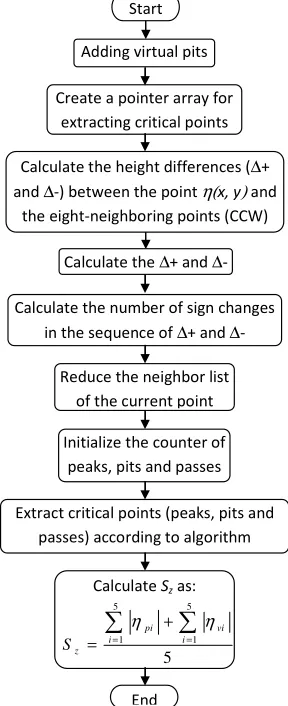
Ten point height of the surface (Sz) is an extreme parameter
defined as the average value of the absolute heights of the five highest peaks and the depths of the deepest pits or valleys within the sampling area. A problem arises when calculating this parameter with digital computers, i.e. th
summits and valleys of areal topographic data [21].
horizontal and vertical Vertical Resolution (µm/pixel)
0.9343
tandard specimen measured by a Surftest SJ201-P. standard specimen
Value 2.97 11.3 3.37 11.72 5.15 102.5 15 lowest valley, R3z (µm) 10.97
m) 97
m) 98
ALGORITHMS
Eight parameters for characterizing the amplitude are specified here. Amplitude were calculated according to . At first, a least square mean applied so that the sum of the squares of asperity departures from this plane is a minimum. The least squares mean plane is unique for a given surface and it minimizes the other planes. For , its linear or first order least squares where are the coefficients to be solved from the given The calculated roughness parameters in
(Sa), root mean
kurtosis (Sku), ten-point
, Minimum Valley (Sv),
is an extreme parameter defined as the average value of the absolute heights of the five highest peaks and the depths of the deepest pits or valleys within the sampling area. A problem arises when calculating this parameter with digital computers, i.e. the definition of summits and valleys of areal topographic data [21].
Fig. 8. Application of least square mean plane and 3D amplitude parameters calculation.
They are more ambiguous compared with the definition of peaks and valleys of the profile data.
be defined within four nearest neighbors or eight nearest neighbors or contour-based summit. Secondly, the ridges, saddles, valleys and local undulations around the highest summit may adversely affect the ability to find the second and subsequent highest summits. Even for the contour summit, a problem arises as to whether only one summit should be defined on a ridge or not. Although Peucker and Douglas [22]-[24] proposed a method to identify summits, flats, straits and ridges, the algorithm still relies on the size of neighboring area. Thus all the problems in defining the summit are concentrated on the extent of the neighboring area within which a summit should be defined. By using different definitions, the number of summits and
the summits would be different. Anyway, the method of extracting summits, flats, straits and ridges that proposed by Peucker and Douglas, is used in this study as shown in Fig.
Start y c x b z a z c x z b M k N
l l l M k N l M k N l l y y y y x y x x y x x
l K l
M
k N
l k k
K K − − = − − = − − = ∑∑ ∑∑ ∑∑ ∑∑ = = = = = = = = 1 1 1 1 1 ) ( ) , ( ( ( ) ( ) , ( ( ( 1 1 1 End ∑ ∑ ∑ = = = = = = N l N l l M k
k y y
x x
MN z N
M 1 1 1
1 1 1
η(x, y)= z(x, y)-(a+bx+cy)
∑∑
= = = N j M i i a x MN S 1 1 , ( 1 η∑ ∑
= = = N j M i i q x MN S 1 1 2 ( 1 η∑ ∑
= = = N j M i q sk x MNS S 1 1 3 3 ( 1 η∑ ∑
= = = N j M i q ku x S MN S 1 1 4 4 ( 1 η 5 5 1 5 1∑
∑
= = + = i vi i pi z S η ηSp=max(max(η(x, y)
Sv=abs(min(min(η(x, y
St=Sp+Sv
Read η(x, y)
. Application of least square mean plane and 3D
They are more ambiguous compared with the definition of peaks and valleys of the profile data. Firstly, a summit may be defined within four nearest neighbors or eight nearest based summit. Secondly, the ridges, saddles, valleys and local undulations around the highest summit may adversely affect the ability to find the second d subsequent highest summits. Even for the contour-based summit, a problem arises as to whether only one summit should be defined on a ridge or not. Although Peucker and proposed a method to identify summits, e algorithm still relies on the size of neighboring area. Thus all the problems in defining the summit are concentrated on the extent of the neighboring area within which a summit should be defined. By using different definitions, the number of summits and the average height of the summits would be different. Anyway, the method of extracting summits, flats, straits and ridges that proposed by Peucker and Douglas, is used in this study as shown in Fig. 9.
z z − − ) ) ∑ ∑ = N M k l k y x z 1 1 ) , ( (a+bx+cy) j y ) , j
i,y )
j i,y)
j i y
x, )
vi
[image:4.612.71.300.79.238.2] [image:4.612.70.303.282.409.2]Fig. 9. Flowchart of Sz parameter calculation based on
extraction of critical points (23-24).
VII. SYSTEM VERIFICATION
To verify the accuracy of the introduced system, twenty images for different sections in each of the two standard specimens were captured and processed by the SR3DVision
program to extract their roughness profiles and to calculate the 2D roughness parameters. The averages of Ra and Rt for
the forty images were calculated and compared with the actual values of the two standard specimens as shown in Table III. The percentage of differences between the actual and the measured values were within ±4.5%. Table IV shows the calculated three dimensional roughness parameters, obtained by both the third module of the SR3DVision
program and a commercial software, for an area of the standard specimens. A Web-based surface metrology algorithm testing system (http://syseng.nist.gov/VSC/jsp) [25], was used to verify the SR3DVision program. This system includes surface analysis tools and a surface texture specimen database for parameter evaluation and algorithm verification. It was found that the maximum difference between the results of the two software is less than 6.65% for ten-point height of the surface (Sz). This may be due to the
[image:5.612.113.257.51.404.2]method of ten-point height calculation presented here. The difference percentages for the other parameters are ranging from 0 to 3.13%. From the table, the maximum percentage of difference between the two systems does not exceed ±4.8%.
Table III: Actual and calculated roughness parameters for the two standard specimen
S
ta
n
d
ar
d
S
p
ec
im
en
Average roughness Ra (µm)
Maximum peak to valley height Rt (µm)
A
cc
u
ra
cy
(%
)
Actual Ave. Diff.
(%) Actual Ave. Diff.
(%)
[image:5.612.311.543.170.299.2]I 2.97 2.98 ±0.50 11.72 12.10 3.77 ±3.14 II 2.97 2.92 ±1.82 13.21 12.91 4.46 ±2.32 Table IV: Calculated unfiltered 3D roughness parameters of a two standard specimen surfaces
Standard specimen I Standard specimen II SR3DVision Mountain Diff.% SR3DVisionMountainDiff.%
Sa (µ m) 11.26 11.2 0.54 10.43 10.4 0.29 Sq (µ m) 11.97 12 0.25 11.06 11.1 0.36
Ssk 0.052 0.053 1.89 0.033 0.032 3.13
Sku 1.45 1.45 0.00 1.41 1.43 1.40
Sz (µm) 44.53 42.5 4.78 38.21 36.5 4.68 Sp (µ m) 24.68 24.8 0.48 19.66 20 1.70 Sv (µm) 21.64 22.2 2.52 19.39 19.5 0.56
St (µm) 46.31 47 1.47 40.05 41 2.32
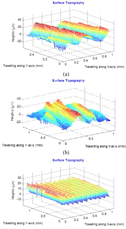
The captured images and the extracted roughness profiles for turned and a milled specimens are shown in Figs. 10 and 11, whereas, the captured images and the extracted roughness profiles for the one standard specimen is shown in Figs. 12. Fig. 13 shows the extracted surface topography of (a) turning (facing), (b) milling, and (c) standard specimen I.
[image:5.612.317.542.389.459.2](a) Original image. (b) Roughness profile . Fig. 10. The captured images and the final roughness profiles for turning specimen (facing).
[image:5.612.314.540.496.557.2](a) Original image. (b) Roughness profile . Fig. 11. The captured images and the final roughness profiles for ground specimen.
(a) Original image. (b) Roughness profile . Fig. 12. The captured images and the final roughness profiles for milled specimen.
VIII. CONCLUSIONS
A non-contact and multi-parameter system for measuring surface roughness has been realized by combining a light
Create a pointer array for extracting critical points
Start
Adding virtual pits
Calculate the ∆+ and ∆-
Calculate the number of sign changes in the sequence of ∆+ and ∆-
Reduce the neighbor list of the current point
End Initialize the counter of
peaks, pits and passes Calculate the height differences (∆+ and ∆-) between the point η(x, y) and
the eight-neighboring points (CCW)
Extract critical points (peaks, pits and passes) according to algorithm
Calculate Sz as:
5
5
1 5
1
∑
∑
= =
+
= i
vi i
pi
z S
η η
0 0.1 0.2 0.3 0.4 0.5 0.6 0.7 0.8 0.9 -10
0 10 20
Travelling along x-axis (mm)
Ir
ri
g
u
la
ri
ty
h
e
ig
h
ts
(µµµµ
m
)
0 0.1 0.2 0.3 0.4 0.5 0.6 0.7 0.8 0.9 -10
-5 0 5 10
Travelling along x-axis (mm)
Ir
ri
g
u
la
ri
ty
h
e
ig
h
ts
(
µµµµ
m
)
0 0.1 0.2 0.3 0.4 0.5 0.6 0.7 0.8 0.9 -5
0 5
Travelling along x-axis (mm)
Ir
ri
g
u
la
ri
ty
h
e
ig
h
ts
(
µµµµ
m
[image:5.612.313.540.600.665.2]sectioning microscope and computer vision system. The vision system has been utilized to capture images for the roughness profiles viewed by light sectioning microscope and save them for further image processing. A program named (SRLSVision) has been specifically written in
process the captured images. Four modules,
graphical user interface (GUI), were developed to extract the roughness profiles from the captured images and to calculate roughness parameters from the extracted profiles.
common surface roughness parameters are calculated by the introduced system. The system was calibrated for both horizontal and vertical resolutions, using
specimens, to calculate the roughness parameters in Metric units. Also, the standard specimens were used to verify t system. In addition, various samples machined by different operations were measured by the introduced system and a stylus instrument and the results showed that the maximum difference between the two systems was within
prove the accuracy of the system.
(a)
(b)
[image:6.612.78.290.280.665.2](c)
Fig. 13. Surface topography of (a) turning (facing), ( and (c) standard specimen I.
REFERENCES [1] T. R. Thomas, Rough surfaces. Longman, Lond
1982, pp. 47-52.
tioning microscope and computer vision system. The vision system has been utilized to capture images for the roughness profiles viewed by light sectioning microscope processing. A program ally written in-house to supported by a were developed to extract the roughness profiles from the captured images and to calculate roughness parameters from the extracted profiles. Most of the surface roughness parameters are calculated by the introduced system. The system was calibrated for both horizontal and vertical resolutions, using two standard , to calculate the roughness parameters in Metric standard specimens were used to verify the system. In addition, various samples machined by different operations were measured by the introduced system and a that the maximum ithin ±4.5%, which
. Surface topography of (a) turning (facing), (b) milling,
Longman, London & New York,
[2] D. J. Whitehouse, Handbook of surface metrology. publishing, Bristol BS1 6NX, UK, 1994, ch . 4. [3] B. J. Griffiths, R. H. Middleton, and B. A.
for the measurement of surface finish -Journal of Production Research, Vol. 32, No. 11 2694.
[4] A. Hertzsch, K. Kröger, and H. Truckenbrodt analysis of turned surfaces by model-based scatterometry,” Engineering, Vol. 26, 2002, pp. 306-313.
[5] B. Dhanasekar, N. Krishna Mohan, Basanta Bhaduri, Ramamoorthy, “Evaluation of surface roughness based on monochromatic speckle correlation using image processing, Precision Engineering, Vol. 32, 2008, pp.
[6] J. C. Wyant, C. L. Koliopoulos, B. Bhushan, “Development of a three-dimensional
profiler,” Journal of Tribology, Vol. 108 /1, 1986,
[7] B. Y. Lee, H. Juan, and S. F. Yu, “A study of computer vision for measuring surface roughness in the turning process,
Journal of Advanced Manufacturing Technology, 295-301.
[8] M. Gupta, and S. Raman, “Machine vision assisted characterization of machined surfaces,” International Journal of Production Research, Vol. 39, No. 4, 2001, pp. 759-784.
[9] E. S. Gadelmawla, “A vision system for surface roughness characterization using the gray level co-occurrence matrix, International, Vol. 37, 2004, pp. 577–588
[10] G. A. Al-Kindi, and B.Shirinzadeh, “
roughness parameters measurement using vision International Journal of Machine Tools & Manufacture, 3-4, 2007, pp. 697-708.
[11] R. Kumar, P. Kulashekar, B. Dhanasekar,
“Application of digital image magnification for surface roughness evaluation using machine vision,” International Journal of Machine Tools & Manufacture, Vol. 45, 2005, pp.
[12] G. Schmaltz, Technische Oberflächenkunde 1936, pp. 5-8.
[13] M. B. Kiran, B. Ramamoorthy and V. Radhakrishnan, surface roughness by vision system,”
machine tools and manufacture, Vol. 38, No. 5
[14] L. Shou-Bin, and Y. Hui-Fen, “Design of a commercial optical instrument for surface roughness measurement,
1995, pp. 190-200.
[15] J. Lewandowski, and J. Desjardins, “Light sectioning with improved depth resolution” Optical Engineering,
2481-2486.
[16] L. Shou-Bin, and Y. Hui-Fen, “Surface roughness measurement by image processing method,” SPIE, Vol. 2101
[17] N. A. Elhamshary, O. B. Abouelatta, E. S. Gadelmawla, I.
Surface roughness measurement using light sectioning method and computer vision techniques, Mansoura Engineering Journal (MEJ), Vol. 29, No. 1, 2003, pp. M.1-M.12
[18] O. Abouelatta and I. Elewa, “Automation of Two Surface Roughness Instrument for Three Texture Assessment,” 9th
IMEKO Symposium Metrology for Quality Control in Production; Surface Metrology for Quality A IMEKO – ISMQC, National Institute of Standards (NIS), 2001, Cairo, Egypt, pp. IV-11- IV-18
[19] ISO 4287:1997+Cor. 1:1998, “Geometrical Product Specifications (GPS) - Surface texture: Profile method
surface texture parameters, 1998.
[20] Surface texture (surface roughness waviness, and lay), An American national standard, The American Society of Mechanical Engineers, ASME B46.1-2002, Revision of ASME B46.1
[21] K. J. Stout, et al. “The development of characterizations of roughness in three dimensions,
behave of the commission of the European communities, Report EUR. 15178 EN, 1993, Part IV.
[22] T. K. Peucker, and D. D. Douglas, “Detection of surface points by local parallel processing of discrete terrain elevation data Computer Graphics and Image Processing,
387.
[23] J. Pfaltz, “Surface Networks,” Geographical Analysis, pp. 77-93.
[24] G. W. Wolf, “A FORTRAN subroutine for cartographic generalization,” Computers and Geosciences
pp.1359-1381.
[25] S. H. Bui, and T. V. Vorburger, “Surface metrology algorithm testing system,” Precision Engineering, Vol. 31,
Handbook of surface metrology. Institute of physics , ch . 4.
A. Wilkie, “Light-scattering - A review,” International Vol. 32, No. 11, 1994, pp.
2683-and H. Truckenbrodt, “Microtopographic based scatterometry,” Precision
ishna Mohan, Basanta Bhaduri, and B. Evaluation of surface roughness based on monochromatic speckle correlation using image processing,”
, pp. 196-206.
J. C. Wyant, C. L. Koliopoulos, B. Bhushan, and D. Basila, imensional noncontact digital optical
Vol. 108 /1, 1986, pp. 1-8.
A study of computer vision for measuring surface roughness in the turning process,” International Journal of Advanced Manufacturing Technology, Vol. 19, 2002, pp.
Machine vision assisted characterization of International Journal of Production Research,
A vision system for surface roughness occurrence matrix,” NDT&E 588.
“An evaluation of surface rement using vision-based data,” International Journal of Machine Tools & Manufacture, Vol. 47, No.
Kumar, P. Kulashekar, B. Dhanasekar, and B. Ramamoorthy, Application of digital image magnification for surface roughness International Journal of Machine
pp. 228–234.
Technische Oberflächenkunde. Springer Verlag, Berlin,
Radhakrishnan, “Evaluation of ” International journal of Vol. 38, No. 5-6, 1998, pp. 685-690. Design of a commercial optical instrument for surface roughness measurement,” SPIE, Vol. 2349,
Light sectioning with improved Vol. 34, No. 8, 1995, pp.
Surface roughness measurement by Vol. 2101, 1993, pp. 1323-1328.
S. Gadelmawla, I. M. Elewa, Surface roughness measurement using light sectioning method and Mansoura Engineering Journal (MEJ),
Elewa, “Automation of Two-Dimensional Surface Roughness Instrument for Three-Dimensional Surface IMEKO Symposium Metrology for Quality Control in Production; Surface Metrology for Quality Assurance, ISMQC, National Institute of Standards (NIS), 24-27 Sept.
Geometrical Product Specifications Surface texture: Profile method – Terms,” Definitions and
Surface texture (surface roughness waviness, and lay), An American The American Society of Mechanical Engineers,
Revision of ASME B46.1-1995
The development of methods for the characterizations of roughness in three dimensions,” Published on behave of the commission of the European communities, Report EUR.
Detection of surface-specific parallel processing of discrete terrain elevation data,” Computer Graphics and Image Processing, Vol. 4, 1975, pp.
375-Geographical Analysis, Vol. 8, 1976,
A FORTRAN subroutine for cartographic Computers and Geosciences, Vol. 17, No. 10, 1991,