PLS Path Modeling with Mode C Computational Experiments

PLS Path Modeling with Mode C

Computational Experiments

Alba Martinez-Ruiz

_{, Tomas Aluja-Banet}

Abstract—Monte Carlo simulations and computa-tional experiments were carried out to study the per-formance of partial least squares (PLS) path modeling with mode C. The empirical results are in line with the theoretical PLS framework. Inner relationships are underestimated and outer relationships overesti-mated.

Keywords: partial least squares, structural equation models, Monte Carlo simulation

1

Introduction

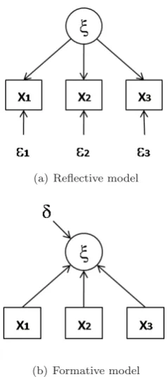
Reflective relationships seek to represent variances and covariances between the manifest variables that are gen-erated or caused by a latent variable. So, observed vari-ables are treated as an effect of unobserved varivari-ables [2]. In a reflective measurement model, the manifest variables are measured with error (Figure 1(a)). Alternatively, for-mative relationships are used to minimize residuals in the structural relationship [9]. Here, manifest variables are treated as forming the unobserved variables, they are presumed to be error–free, and the construct is es-timated as a linear combination of the manifest variables plus a disturbance term (Figure 1(b)). As in this case all variables forming the construct should be considered, the disturbance term represents all those non-modeled causes. Although formative measurement models were first discussed by [4] and [1], and a number of variables can be modeled in a better way through formative rela-tionships, measurement variables have been traditionally modeled in a reflective mode. [9] and [5] pointed out that modeling formative modes using a covariance-based approach may lead to identification problems and Hey-wood cases. So, researchers may tend to define outer models as reflective. However, a number of researchers have pointed out that PLS path modeling overcomes the identification problems that arise when implementing a covariance-based approach [15, 17, 19]. That is because a PLS path modeling algorithm consists of a series of

or-∗_{This research was supported by a grant from the} Univer-sidad Cat´olica de la Ssma. Concepci´on, and the Comisi´on Nacional de Investigaci´on Cient´ıfica y Tecnol´ogica (CONICYT), Chile. A. Martinez-Ruiz and T. Aluja-Banet are with Techni-cal University of Catalonia, Department of Statistics and Oper-ations Research, Jordi Girona 1-3, C5, 08034 Barcelona, Spain. Tel/Fax: 93-401-7986/5855 E-mails: [email protected], [email protected].

dinary least squares (OLS) analysis. From a component-based approach, and “because the off-diagonal elements are not among the unknown parameters of the model and because the unobservables are explicitly estimated, there are no identification problems for recursive PLS models” [9, p. 443].

In Wold’s PLS approach, a construct is completely determined by a linear combination of its indicators [17, 18, 19]. The procedure usually uses a Mode A or Mode B to model a structural equation model (SEM). Mode A or simple regression if the SEM includes reflective outer models. Mode B or multiple regression if formative outer models are included. However, “the algorithm is called PLS Mode C if each of Modes A and B is chosen at least once in the model” [18, p. 10]. To the best of our knowledge, there are only a small number of published articles that examine the performance of PLS path mod-eling algorithm in the presence of formative outer models, and they are not conclusive. Findings by [3] and [13] are quite different. For instance, Cassel et al. found that measurement relationships in formative outer models are overestimated, while Ringle et al. found that these rela-tionships are underestimated. Thus, this paper aims to provide evidence regarding how well PLS path modeling performs if formative exogenous outer models are mod-eled using PLS Mode B and reflective endogenous latent variables are modeled using PLS Mode A. That is, PLS path modeling with mode C.

2

PLS Path Modeling

The PLS path modeling procedure –presented by Ger-lach, Kowalski, and Wold in 1979– is a soft modeling technique and a data analytic tool for estimating struc-tural equation models (SEM) and building a sequence of latent variables. PLS path modeling first estimates the unobservable variables and then the parameters with an aim toward maximizing the total variance and mini-mizing residuals of endogenous models regardless of the covariances among manifest variables. The structural or inner model describes relationships among constructs

ξi by means of multiple regressions (Equation 1). ξi

(a) Reflective model

(b) Formative model

Figure 1: Reflective and formative measurement models (focus on component-based approach)

E(ξ_j/ξ_i) = _iβ_jiξ_i, that is, there is no linear relation-ship between predictor and residual. This condition im-plies thatE(ν_j/∀ξ_i) = 0, andcov(ν_j, ξ_i) = 0.

ξj=βj0+

i

βjiξi+νj (1)

Manifest variables revealing or reflecting the effect of a construct are modeled as indicators of it in a reflective measurement model. Each manifest variable x_jh is re-lated by simple ordinary least squares regression with the underlying construct ξ_j (Equation 2). The loadings λ_h determine the extent to which each indicator reflects a construct;ξ_j is a common factor with mean m, standard deviation one and it is indirectly observable by the man-ifest variables. The condition imposed by Herman Wold is predictor specification, E(x_h/ξ) = λ_h0 +λ_hξ. This condition implies that_h has zero mean, and it is uncor-related with ξ_j. Moreover, the basic design of Herman Wold assumes that the covariance matrices of all _j are diagonal. As in a reflective model, where all the indica-tors of the block of variables reflect the same construct, there should be high collinearity among these variables. That is, the blocks of variables must be one-dimensional.

xjh=λjh0+λjhξj+jh (2)

The latent variable is formed by a set of manifest vari-ables as a linear function of them plus a residual in

for-mative outer models (Equation 3). The weightsπ_h de-termine the extent to which each indicator contributes to the formation of the constructs. Each block of manifest variables may be multidimensional, and multicollinear-ity among indicators is not a necessary constraint. The condition imposed by Herman Wold is predictor

specifica-tionE(ξ/X₁, ..., X_pj) =_hπ_hx_h. This condition implies

that the residualδhas a zero mean, and it is uncorrelated with the manifest variablesx_h. Since each construct is formed by a linear combination of the manifest variables, the sign of each weightπ_h should be the same sign as the correlation betweenx_handξ [15].

ξj=

h

πjhxjh+δj (3)

2.1

PLS path modeling algorithm

The PLS path modeling algorithm is structured in three stages [17, 18, 19]. The first stage computes the case values of the latent variables; the second stage focuses on the inner and outer relationships; and in the third stage, location parameters of the latent variables, λ_jh0 andβ_j0, are estimated. Only the first stage is iterative. The algorithm for Wold’s procedure is as follows.

The first stage. The algorithm starts choosing an ar-bitrary weight vector –outer weights– to first relate each latent variable with their own manifest variables. Usually this vector is a vector of ones. Each standardized latent variableY_j–zero mean, unit variance– is computed as an exact linear combination of their own centered manifest variables:

Yj =

wjhxjh (4)

wherew_jh are called the outer weights.

An auxiliary latent variable Z_j is introduced as a coun-terpart to the variable Y_j. Each Z_j is computed as a weighting sum of the latent variables which is related to:

Zj ∝

ejiYi (5)

where e_ji are called the inner weights. There are three different weighting schemes that may be used to compute

eji: the centroid, the factorial and the path weighting

schemes. The first was introduced by Wold, and the last two by [11]. The simplest scheme is the centroid scheme where the e_ji are equal to the signs of the correlations between Y_j and the Y_i’s. The inner weights are equal to the correlation betweenY_j andY_i when the factorial scheme is considered. The inner weights in a path weight-ing scheme are (a) equal to the regression coefficients of

Yi in the multiple regression ofYjon all theYirelated to

the predecessor ofY_j, or (b) are equal to the correlation between the successor ofY_i andY_j.

itera-tive process, these weights are used to estimate all latent variable scores as a linear combination of their own indi-cators. The procedure considers two ways of recomputing the outer weights, depending on the reflective or forma-tive nature of the outer models: mode A and mode B. Usually, mode A is considered for recomputing the outer weights when outer models are reflective, and mode B is considered for recomputing the outer weights when outer models are formative. However, this rule is not manda-tory. Depending on models, data characteristics and also the researcher’s discretion, one mode or another will be more appropriate for a particular case. For mode A, the

wjh is the regression coefficient of Zj in the simple

re-gression ofx_jhon the inner estimation ofZ_j:

wjh=cov(xjh, Zj) (6)

For mode B, the vectorw_jof weightsw_jhis the vector of the regression coefficient in the multiple regression ofZ_j on the manifest variables (x_jh−x_jh) related to the same latent variableZ_j:

wj = (XjXj)−1XjZj (7)

The first stage is iterated until convergence.

The second stage. Once the algorithm converges, the latent variable scores estimated in stage 1 are used to es-timate the inner and outer relationships by ordinary least squares regression without location parameters. If reflec-tive blocks of variables are modeled, simple regression is used to estimate loadings (Equation 2). If formative blocks of variables are modeled, weights are estimated by ordinary multiple regression (Equation 3).

The third stage. The third stage focus on estimation of the location parameters, and the values of π_jh0 and

βj0(Equation 1).

3

Monte Carlo Simulation Study

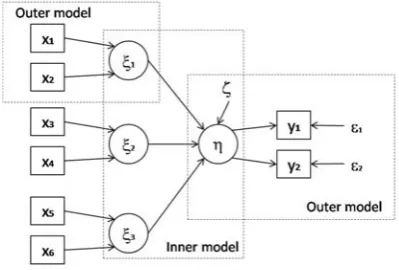
A Monte Carlo simulation study was designed to ana-lyze the performance of PLS path modeling with mode C [12, 10]. The underlying population model considered a simple structure with three formative exogenous con-structs and one reflective endogenous latent variable (Fig-ure 2). Models with two, four, six and eight indicators per construct, and four different samples sizes (50, 100, 250, 500) were studied. Five hundred random data sets were generated for each of the 4×4 cells of the two-factor design. PLS path modeling with centroid scheme –as de-scribed in [15]– and bootstrapping were performed in R-project [14]. Five hundred replications (t) were made for each cell in the design. Results are provided in terms of the mean bias (accuracy, 1_tt_i=1E[θ_i]−θ) and mean relative bias (MRB= 100∗ 1_tt_i=1θ−E[θi]

θ , [7]).

The data were generated from a component-based model. We began generating standardized manifest variablesx_jh

Figure 2: Inner and outer models of the simulated setups; outer models consider two, four, six, and eight indicators per construct.

for each formative outer model as independent normal data. Once the manifest variables were generated, we computed the exogenous constructs ξ_j and the endoge-nous latent variable η, so that the variance of the un-observable variables is one. The generated exogenous constructs are not collinear. The endogenous latent vari-able was calculated as linear combination of the exoge-nous constructs plus a disturbance term. Disturbance terms were computed as random normal data with a zero mean and the corresponding standard deviation. They were distributed independently of unobservable variables. Standardized observed variablesy_iof reflective measure-ment models were generated as independent normal data. Errors of the reflective relationships were computed as random normal data with a zero mean and the corre-sponding standard deviation; they were also uncorrelated with the latent variable. To set the true population pa-rameters for the models, we took into account different combinations of permissible values so as to see whether they are recovered by the PLS path modeling algorithm. Table 1 shows the true population values of weights, path coefficients and loadings. We consider large values for all the true loadings, at least 0.7 in the case of two manifest variables per construct. This ensures the unidimensional-ity of the block of variables and it satisfies the condition imposed by the PLS path modeling algorithm.

4

Results

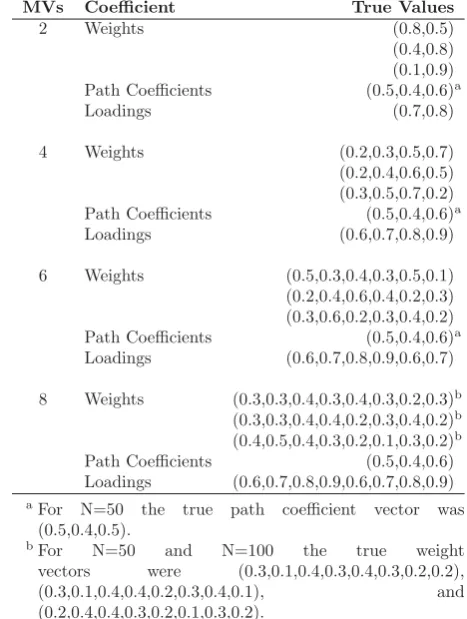
increas-Table 1: Vector of true population values for weights, path coefficients and loadings; cases for two, four, six and eight indicators in each outer model.

MVs Coefficient True Values

2 Weights (0.8,0.5)

(0.4,0.8) (0.1,0.9) Path Coefficients (0.5,0.4,0.6)a

Loadings (0.7,0.8)

4 Weights (0.2,0.3,0.5,0.7)

(0.2,0.4,0.6,0.5) (0.3,0.5,0.7,0.2) Path Coefficients (0.5,0.4,0.6)a

Loadings (0.6,0.7,0.8,0.9)

6 Weights (0.5,0.3,0.4,0.3,0.5,0.1) (0.2,0.4,0.6,0.4,0.2,0.3) (0.3,0.6,0.2,0.3,0.4,0.2) Path Coefficients (0.5,0.4,0.6)a Loadings (0.6,0.7,0.8,0.9,0.6,0.7)

8 Weights (0.3,0.3,0.4,0.3,0.4,0.3,0.2,0.3)b (0.3,0.3,0.4,0.4,0.2,0.3,0.4,0.2)b (0.4,0.5,0.4,0.3,0.2,0.1,0.3,0.2)b Path Coefficients (0.5,0.4,0.6) Loadings (0.6,0.7,0.8,0.9,0.6,0.7,0.8,0.9) a_{For N=50 the true path coefficient vector was}

(0.5,0.4,0.5).

b_{For N=50 and N=100 the true weight} vectors were (0.3,0.1,0.4,0.3,0.4,0.3,0.2,0.2), (0.3,0.1,0.4,0.4,0.2,0.3,0.4,0.1), and (0.2,0.4,0.4,0.3,0.2,0.1,0.3,0.2).

ing the sample size or increasing the number of manifest variables in all the simulated cases.

Simulations performed by [6] for PLS models with re-flective relationships showed that, by themselves, neither the number of indicators nor the sample size substan-tively improve the quality of the estimates. Rather, it is necessary to increase both factors at the same time for an improvement in the quality of the estimates. Here, the simulations for PLS models with formative blocks of variables render the same aforementioned result. So, PLS path modeling is consistent and consistent at large. Nev-ertheless –and recalling that PLS algorithm computes the latent variables as an exact linear combination of the ob-served variables– the results suggest that estimates will improve by increasing the sample size more than increas-ing the number of observable variables, dependincreas-ing on the correlations between manifest variables. So, the re-searcher may suspect the type of relationship that she expects to find.

As can be seen in Figure 3(b), the estimates of loadings are very close to the true values in all cases, regardless of the sample sizes and number of manifest variables per construct. PLS path modeling overestimates the

popula-0 100 200 300 400 500

−20

0

10

20

Case C − Weight = 0.5 (500 runs)

Sample size

MRB (%)

2 MVs 4 MVs

6 MVs 8 MVs

(a) MRB for a weight of 0.5

0 100 200 300 400 500

−30

−20

−10

0

Case C − Loading = 0.7 (500 runs)

Sample size

MRB (%)

2 MVs 4 MVs 6 MVs 8 MVs

(b) MRB for a loading of 0.7

Figure 3: Mean relative bias of a weight and a loading. Highlighting the influence of the sample size and the num-ber of indicators per construct.

tion values. Moreover, according to the results, a higher number of manifest variables seems to be more important than a higher sample size for decreasing the bias of the estimates in reflective outer models. This is in contrast with the formative relationships and coincides with the results found by other researchers [6]. This is clearly seen in Figure 3(b) where the mean relative bias for a loading of 0.7 strongly decreases when the number of indicators increases. So, this confirms that PLS estimates are con-sistent at large [6, 18].

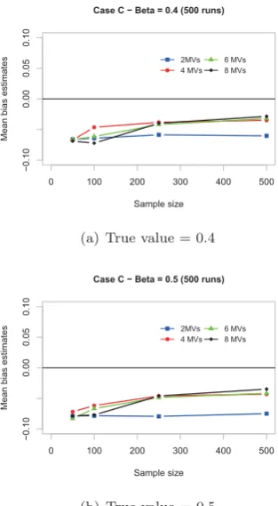
Results for estimates of inner relationships are quite con-clusive. Figure 4 allows us to see how an increase in both the number of manifest variables and the sample size re-duces the mean bias of path coefficients for all assumed true values. The algorithm underestimates the true path coefficients in all the analyzed cases. As the sample size increases, the estimates increasingly approach the true values and the biases decrease.

0 100 200 300 400 500

−0.10

0.00

0.05

0.10

Case C − Beta = 0.4 (500 runs)

Sample size

Mean bias estimates

2MVs 4 MVs

6 MVs 8 MVs

(a) True value = 0.4

0 100 200 300 400 500

−0.10

0.00

0.05

0.10

Case C − Beta = 0.5 (500 runs)

Sample size

Mean bias estimates

2MVs 4 MVs

6 MVs 8 MVs

(b) True value = 0.5

Figure 4: Mean bias of path coefficients. Highlighting the influence of the sample size and the number of indicators.

size does.

Summing up, in all analyzed cases, the results obtained are better when each outer model considers more mani-fest variables per construct. However, it is worth noting that the estimates are shown to be quite accurate and precise when the measurement models include only two indicators per construct. This suggests that PLS path modeling may be a robust alternative when estimating structural equation models with formative relationships and few indicators per construct.

5

Conclusions

For the studied model, the findings suggest that PLS path modeling offers a way to build “proper indices” for unob-servable variables and to estimate the relationships be-tween them. The procedure shows a tendency to over-estimate outer relationships and underover-estimate inner re-lationships. It is worth noting that the estimates are shown to be robust when the measurement models in-clude only two indicators per construct. It is true that when the number of observed variables and sample size increase, the quality of the PLS path modeling estimates increases. But when few indicators and a small sample size are considered, we can obtain acceptable estimates of the parameters. [16] have noted the same behavior in a reflective block of variables with two indicators.

Fi-nally, we think that the model simulated here represents a number of models that can be studied in real-world applications: those in which formative exogenous outer models are modeled using PLS Mode B and reflective en-dogenous latent variables are modeled using PLS Mode A. That is, PLS Mode C, in terms of Wold’s approach.

References

[1] Blalock, H. Causal Inferences in Non-experimental Research, University of North Carolina Press, Chapel Hill, 1964.

[2] Bollen, K., Lennox, R., “Conventional Wisdom on Measurement: A Structural Equation Perspective,” Psychological Bulletin, V110, N2, pp. 305-314, 1991.

[3] Cassel, C., Hackl, P., Westlund, A., “Robustness of Partial Least-Squares Method for Estimating La-tent Variable Quality Structures,” Journal of Ap-plied Statistics, V26, N4, pp. 435-446, 1999.

[4] Curtis, R., Jackson, E., “Multiple Indicators in Sur-vey Research,” The American Journal of Sociology, V68, N2, pp. 195-204, 1962.

[5] Chin, W.W., “Issues and Opinion on Structural Equation Modeling,”MIS Quarterly, V22, N1, 1998.

[6] Chin, W. W., Newsted, P. R., “Structural Equation Modeling Analysis with Small Samples using Partial Least Squares,”Statistical Strategies for Small Sam-ple Research, Hoyle, R. H. (ed), Sage Publications, California, pp. 307-341, 1999.

[7] Chin, W. W., Marcolin, B. L., Newsted, P. R., “A Partial Least Squares Latent Variable Model-ing Approach for MeasurModel-ing Interaction Effects: Re-sults from a Monte Carlo Simulation Study and an Electronic-mail Emotion/Adoption Study,” In-formation Systems Research, V14, N2, pp. 189-217, 2003.

[8] Dijkstra, T., “Latent Variables and Indices: Herman Wold’s Basic Design and Partial Least Squares,” Handbook of Partial Least Squares: Concepts, Meth-ods and Applications, Esposito Vinzi, V., Chin, W. W., Henseler, J., Wang, H. (eds), Springer, Heidel-berg, 2010.

[9] Fornell, C., Bookstein, F. L., “Two Structural Equa-tion Models: LISREL and PLS Applied to Consumer Exit-Voice Theory,”Journal of Marketing Research, V19, N4, pp. 440, 1982.

[10] Gentle, J.,Random Number Generation and Monte Carlo Methods, Springer, New York, 2003.

[12] Paxton, P., Curran, P., Bollen, K., Kirby, J., Chen, F., “Monte Carlo Experiments: Design and Imple-mentation,” Structural Equation Modeling: A Mul-tidisciplinary Journal, V8, N2, pp. 287-312, 2001.

[13] Ringle, C.M., G¨otz, O., Wetzels, M., Wilson, B., “On the Use of Formative Measurement Specifica-tions in Structural Equation Modeling: A Monte Carlo Simulation Study to Compare Covariance– based and Partial Least Squares Model Estimation Methodologies,” Maastricht University, METEOR Research Memoranda RM/09/014, 2009.

[14] R Development Core Team, “R: A Language and Environment for Statistical Computing,” R Foun-dation for Statistical Computing, Vienna, Austria, http://www.R-project.org, 2007.

[15] Tenenhaus, M., Esposito Vinzi, V., Chatelin, Y. M., Lauro, C., “PLS Path Modeling,” Computational Statistics & Data Analysis, V48, pp. 159-205, 2005.

[16] Vilares, M., Almeida, M., Coelho, P., “Compari-son of Likelihood and PLS Estimators for Struc-tural Equation Modeling: A Simulation with Cus-tomer Satisfaction Data,”Handbook of Partial Least Squares: Concepts, Methods and Applications, Es-posito Vinzi, V., Chin, W. W., Henseler, J., Wang, H. (eds), Springer, Heidelberg, 2009.

[17] Wold, H., “Model Construction and Evaluation when Theoretical Knowledge is Scarce: Theory and Application of Partial Least Squares,” Evaluation of Econometric Models, J. Kmenta, J., Ramsey, G. (eds), Academic Press, New York, pp. 47-74, 1980.

[18] Wold, H., “Soft Modeling: The Basic Design and Some Extensions,” Systems Under Indirect Obser-vation, J¨oreskog, K. G., Wold, H. (eds), North-Holland, Amsterdam, pp. 1-54, 1982.