Capturing and Treating Unobserved Heterogeneity by Response Based Segmentation in PLS Path Modeling. A Comparison of Alternative Methods by Computational Experiments

C

APTURING AND

T

REATING

U

NOBSERVED

H

ETEROGENEITY

BY

R

ESPONSE

B

ASED

S

EGMENTATION IN

PLS P

ATH

M

ODELING

.

A C

OMPARISON OF

A

LTERNATIVE

M

ETHODS BY

C

OMPUTATIONAL

E

XPERIMENTS

V

E

V

, C

M. R

,

S

S

, L

T

© ESSEC / CTD - Centr e de R echer che / 0 4090 71 232 GROUPE ESSEC

centre de recherche / RESEARCH CENTER AVENUE BERNARD HIRSCH

BP 50105 CERGY

95021 CERGY PONTOISE CEDEX FRANCE

TéL. 33 (0)1 34 43 30 91 FAX 33 (0)1 34 43 30 01

[email protected]

essec business school.

établissements privés d’enseignement supérieur, association loi 1901,

accréditéS aacsb international - the association TO ADVANCE COLLEGIATE SCHOOLS OF BUSINESS,

accrédités EQUIS - the european quality improvement system, affiliés à la chambre de commerce et d’industrie

de versailles val d’oise - yvelines. Pour tous renseignements :

• Centre de Recherche/Research Center

Tél. 33 (0)1 34 43 30 91 [email protected]

• Visitez notre site www.essec.fr

DR 07019

Capturing and Treating Unobserved Heterogeneity

by Response Based Segmentation in PLS Path Modeling.

A Comparison of Alternative Methods by Computational Experiments

Vincenzo ESPOSITO VINZI

Christian M. RINGLE

Silvia SQUILLACCIOTTI

Laura TRINCHERA

Abstract:

Segmentation in PLS path modeling framework results is a critical issue in social sciences. The

assumption that data is collected from a single homogeneous population is often unrealistic. Sequential

clustering techniques on the manifest variables level are ineffective to account for heterogeneity in path

model estimates. Three PLS path model related statistical approaches have been developed as solutions

for this problem. The purpose of this paper is to present a study on sets of simulated data with different

characteristics that allows a primary assessment of these methodologies.

Keywords:

Partial Least Squares, Path Modeling, Unobserved Heterogeneity

Résumé :

De nos jours, les problématiques liées à la recherche d’hétérogénéité parmi les unités sont devenues

critiques dans le cadre des modèles structurels PLS, notamment dans les sciences sociales. L’hypothèse

de base de cette méthode, selon laquelle les données proviennent d’une population unique et homogène,

s’avère souvent peu réaliste. Les techniques de classification séquentielles sur les variables manifestes

sont fréquemment peu efficaces lorsque l’on veut découvrir l’hétérogénéité dans les estimations des

paramètres des modèles structurels. Trois approches statistiques ont été développées comme solutions à

ce problème dans le cadre des méthodes PLS. L’objectif de ce papier est de présenter une étude sur des

jeux de données simulées, ayant différentes caractéristiques permettant une première évaluation des

méthodes décrites. Par ces jeux de données, nous allons illustrer l’intérêt de découvrir l’hétérogénéité

latente dans les applications des modèles structurels PLS, décrire les caractéristiques de chaque

méthode, en comparer les points forts et les points faibles, et découvrir des aspects méthodologiques qui

n’ont pas encore été traités. Ces contributions pourront aider chercheurs et praticiens à mieux

comprendre les résultats parfois ambigus des modèles PLS, afin de parvenir à des conclusions

analytiques plus efficaces.

Mots-clés :

Partial Least Squares, Path Modeling, Unobserved Heterogeneity

Response Based Segmentation in PLS Path Modeling

A Comparison of Alternative Methods by Computational Experiments

Vincenzo Esposito Vinzi · Christian M. Ringle · Silvia Squillacciotti · Laura Trinchera

Abstract Segmentation in PLS path modeling framework results is a critical issue in social sciences. The assumption that data is collected from a single homogeneous population is often unrealistic. Sequential clustering techniques on the manifest variables level are inef-fective to account for heterogeneity in path model estimates. Three PLS path model related statistical approaches have been developed as solutions for this problem. The purpose of this paper is to present a study on sets of simulated data with different characteristics that allows a primary assessment of these methodologies. We thereby illustrate the requirement to un-cover unobserved heterogeneity in PLS path model applications, reveal the capabilities of each approach to deal with that issue, compare their strength and weaknesses, and provide methodological implications that have not been addressed, yet. These contributions are par-ticularly important for researchers and practitioners to further differentiate ambiguous PLS path modeling results on the aggregate data level in order to originate effective analytical conclusions.

Keywords Partial Least Squares·Path Modeling·Segmentation·FIMIX-PLS· PLS-TPM·REBUS-PLS

Vincenzo Esposito Vinzi ESSEC Business School,

Department of Information Systems & Decision Sciences (SID), Avenue Bernard Hirsch, B.P. 50105,

95021 Cergy-Pontoise Cedex, France Tel.: +33 1 34.43.36.56

Fax: +33 1 34.43.36.91 E-mail: [email protected] Christian M. Ringle University of Hamburg,

Faculty of Business, Economics and Social Sciences, Von-Melle-Park 5, 20146 Hamburg, Germany Silvia Squillacciotti

Electricit´e de France, Research & Development, 1 Avenue du G´en´eral de Gaulle, 92141 Clamart, France Laura Trinchera

University of NaplesFederico II, Department of Mathematics and Statistics,

1 Introduction

Structural Equation Modeling (SEM) and Latent Variable Path Modeling (LVP) are used to measure complex cause effect relationships (Marcoulides and Saunders, 2006; Chin, 1998). Covariance Based Structural Equation Modeling (CBSEM; J¨oreskog, 1978; Rigdon, 1998) and Partial Least Squares analysis (PLS; Lohm¨oller, 1989; Tenenhaus et al., 2005) constitute the two corresponding statistical techniques for estimating causal models. Wold’s 1982 basic PLS design or basic method of soft modeling is rather a distinctive than alternative approach compared to CBSEM (Fornell and Bookstein, 1982). Soft modeling refers to the ability of PLS to be more flexible in handling various modeling problems in situations where it is difficult or impossible to meet the hard assumptions of more traditional multivariate statis-tics. Within this context, ”soft” is only attributed to distributional assumptions and not to the concepts, the models or the estimation techniques (Lohm¨oller, 1989). Applications of PLS path modeling are well established in academic literature. Recognizable examples in the management sciences discipline are Fornell et al. (1985, 1990); Gray and Meister (2004); Venkatesh and Agarwal (2006).

There are at least three critical issues that have received little or no attention in prior work. First, analyses in a PLS path modeling framework usually do not address the problem of heterogeneity. The failure to account for heterogeneity leads to ambiguous PLS path modeling results and, thus, to conclusions that are incomplete and ineffective.

Second, statistical instruments that extent and complement the PLS approach are not well developed. Especially advances towards analytical methods for clustering data have lagged behind their need in applications. A first approach is to test if data on the manifest variables level belongs to a finite number of clusters by sequential segmentation strategies such as K-means or tree clustering. These methods, however, cannot account for hetero-geneity in the relationships between latent variables and are improper for forming groups of data with distinctive path model estimates (Jedidi et al., 1997). Alternatively, theoretical knowledge allows to analyze the effect of moderating factors (Henseler and Fassott, 2007). This kind of approach only accounts for heterogeneity of a limited number of relationships in the path model and is restricted to the existence of suitable moderating variables.

As a consequence of these limitations in existing methodologies, PLS path modeling requires complementary techniques for response based segmentation such as Finite Mixture Partial Least Squares (FIMIX-PLS; Hahn et al., 2002), Partial Least Squares Typological Path Modeling (PLS-TPM; Squillacciotti, 2007) and REsponse Based Units Segmetation (REBUS; Esposito Vinzi et al., 2007).

Third, knowledge is limited about the capabilities of all these methods. The systematical application of these methodologies to identify and effectively treat unobserved heterogeneity in the path model by segmentation has not been evaluated thus far. In addition, literature does not present a comparison of the methodologies and a critical analysis of their strengths and weaknesses. The failure to account for these issues entails uncertainty about the applicability of FIMIX-PLS, PLS-TPM and REBUS-PLS to analyze PLS path modeling estimates in particular research situations.

In view of these deficiencies, the primary contribution of this article is to provide an ini-tial assessment if FIMIX-PLS, PLS-TPM and REBUS-PLS reliably identify clusters with distinctive path model relationships. We therefore simulate different kinds of data for nu-merical PLS path modeling examples. The simulation study allows us to evaluate the qual-ity of results and, thus, the capabilities of each methodology under systematically changed data constellations. A comparison of the outcomes exposes strengths and weaknesses of each approach. These analyses finally substantiate the requirement and applicability of the

FIMIX-PLS, the PLS-TPM and the REBUS-PLS as analytical extensions and standard test procedures for PLS path modeling.

The findings of our study are particularly important for researchers and practitioners to confirm that PLS path modeling estimates are not affected by heterogeneity in the path model. Outcomes on the aggregate data level may otherwise be inadequate and require seg-mentation. FIMIX-PLS, PLS-TPM and REBUS-PLS indicate how to treat that problem by forming groups of data. Researchers and practitioners can exploit these PLS response based segmentation techniques to assure that results on the aggregate data level are not affected by unobserved heterogeneity in the path model estimates. Otherwise, FIMIX-PLS, PLS-TPM abd REBUS-PLS indicate how to treat that problem by forming groups of data. A multigroup PLS path analysis (Chin and Dibbern, 2007) on the finally established segments provides evidence if segment specific estimates are significantly different. In this case, re-searchers or practitioners obtain supplementary analytical results to further differentiate and render more precisely their conclusions.

The remainder of this article is organized as follows. The next section introduces FIMIX-PLS, PLS-TPM and REBUS-FIMIX-PLS, followed by a section about the design of this study and data simulation. Then, numerical examples allow us to demonstrate the requirement of identifying and treating heterogeneity in the path model estimates. They also provide a means of assessing and substantiating the FIMIX-PLS, the PLS-TPM and the REBUS-PLS approaches and permit an initial comparison of segmentation results. The final section concludes this article with essential implications for PLS path modeling and directions of future research.

2 Response Based Segmentation Techniques for PLS Path Modeling 2.1 Finite Mixture Partial Least Squares

2.1.1 Methodology and Algorithm

Distinctive PLS path model estimates for groups of data may be concentrated in the rela-tionships between latent variables. FIMIX-PLS is a methodology that has been developed by Hahn et al. (2002) to capture this kind of heterogeneity for a pre-determined number ofK

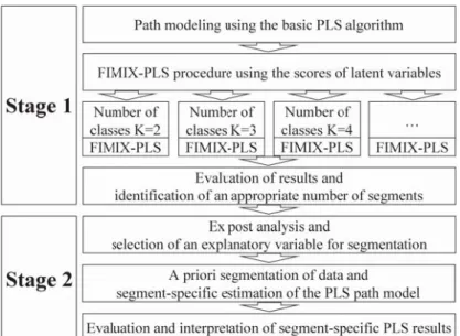
latent classes. A comprehensive FIMIX-PLS application involves the two stages in Figure 1 (Ringle et al., 2007).

In the first stage of FIMIX-PLS, a path model is estimated by using the PLS algorithm for LVP and (empirical) data for manifest variables in the outer measurement models. The resulting scores for latent variables in the inner path model are then employed to run the FIMIX-PLS algorithm and is a key issue regarding the methodological advantages and dis-advantages. On the one hand, the use of latent variable scores allows generally apply FIMIX-PLS in FIMIX-PLS path models (Ringle et al., 2007) regardless whether measurement models of latent variables are operationalized as formative (Diamantopoulos and Winklhofer, 2001) or reflective (Gerbing and Anderson, 1988). On the other hand, the methodology does not directly include detection of heterogeneity in the outer PLS path models.

Equation 1 expresses a modified presentation of the relationships (Table 1 provides a description of all of the symbols used in the equations presented in this paper):

Fig. 1 Analytical Steps of FIMIX-PLS

Segment-specific heterogeneity of path models is concentrated in the estimated rela-tionships between latent variables. FIMIX-PLS captures this heterogeneity and calculates the probability of each observation so that it fits into each of the pre-determinedKnumbers of classes. The segment-specific distributional function is defined as follows, assuming that ηiis distributed as a finite mixture of conditional multivariate normal densitiesfi|k(·):

ηi∼ K

∑

k=1

ρkfi|k(ηi|ξi,Bk,Γk,Ψk) (2)

Substituting fi|k(ηi|ξi,Bk,Γk,Ψk)results in the following equation:

ηi∼ K

∑

lnL=

∑

i

∑

zikln(f(ηi|ξi,Bk,Γk,Ψk)) +

∑

i

∑

zikln(ρk) (4)

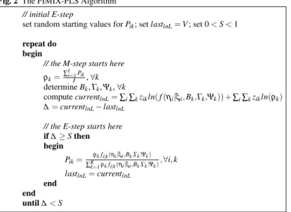
An EM-formulation of the FIMIX-PLS algorithm (Figure 2) is used for statistical com-putations to maximize the likelihood and to ensure convergence in this model. The expecta-tion of Equaexpecta-tion 4 is calculated in the E-step, wherezikis 1 if subjectibelongs to classk(or 0

otherwise). The segment sizeρk, the parametersξi,Bk,ΓkandΨkof the conditional

probabil-ity function are stated (as results of the M-step), and provisional estimates (expected values),

E(zik) =Pik, forzikare computed in the E-step according to Bayes’ theorem (Barnard, 1958,

Table 1 Explanation of Symbols FIMIX-PLS

Am number of exogenous variables as regressors in regressionm

am exogenous variableamwitham=1,...,Am

Bm number of endogenous variables as regressors in regressionm

bm endogenous variablebmwithbm=1,...,Bm

γammk regression coefficient ofamin regressionmfor latent classk

βbmmk regression coefficient ofbmin regressionmfor latent classk

τmk ((γammk),(βbmmk))vector of the regression coefficients

ωmk cell(m×m)ofΨk

c constant factor

fi|k(·) probability for caseigiven a latent classkand parameters(·)

I number of cases or observations

i case or observationiwithi=1,...,I

J number of exogenous latent variables

j exogenous latent variablejwithj=1,...,J

K number of latent classes

k latent class or segmentkwithk=1,...,K

M number of endogenous latent variables

m endogenous latent variablemwithm=1,...,M

Nk number of free parameters defined as(K−1) +KR+KM

Pik probability of membership of caseito latent classk

R number of predictor variables of all regressions in the inner model

S stop or convergence criterion

V large negative number

Xmi case values of the regressors for regressionmof individuali

Ymi case values of the regressant for regressionmof individuali

zik zik=1, if the caseibelongs to latent classk;zik=0 otherwise

ζi random vector of residuals in the inner model for casei

ηi vector of endogenous latent variables in the inner model for casei

ξi vector of exogenous latent variables in the inner model for casei

B M×Mpath coefficient matrix of the inner model

Γ M×Jpath coefficient matrix of the inner model

∆ difference ofcurrentlnLandlastlnL

Bk M×Mpath coefficient matrix of the inner model for latent classk

Γk M×Jpath coefficient matrix of the inner model for latent classk

Ψk M×Mmatrix for latent classkcontaining the regression variances

ρ (ρ1,...,ρK), vector of theKmixing proportions of the finite mixture

ρk mixing proportion of latent classk

PLS-TPM

ξm∗ target endogenous latent variable

Pm∗ number of manifest variables in them∗-th target block

v2

ipm∗k residual of the redundancy model for thei-th observation

in thek-th latent class, corresponding to them∗-th target block

Rd(ξm∗,ypm∗) redundancy index for the target endogenous manifest variables for groupk REBUS

Q total number of latent variables, endogenous and

exogenous ones withQ=J+M

ξq generic latent variable

ξj generic exogenous latent variable

ξm generic endogenous latent variable

P total number of manifest variables

Pq number of manifest variables in theq-th block, with∑Qq=1Pq=P

xpq generic manifest variable in theq-th block

eipqk measurement residual for thei-th observation in thek-th latent class,

corresponding to thep-th manifest variable in theq-th block, i.e. the communality residuals

fimk the structural residual for thei-th observation in thek-th latent class,

corresponding to them-th endogenous block

Fig. 2 The FIMIX-PLS Algorithm

// initial E-step

set random starting values forPik; setlastlnL=V; set 0<S<1

repeat do begin

// the M-step starts here ρk=∑ I i=1Pik I ,∀k determineBk,Γk,Ψk,∀k computecurrentlnL=∑i∑kzikln(f(ηi|ξi,Bk,Γk,Ψk)) +∑i∑kzikln(ρk) ∆=currentlnL−lastlnL

// the E-step starts here if_∆≥Sthen begin Pik= ρk fi|k(ηi|ξi,Bk,Γk,Ψk) ∑K k=1ρkfi|k(ηi|ξi,Bk,Γk,Ψk),∀i,k lastlnL=currentlnL end end until∆<S

Equation 4 is maximized in the M-step. This part of the FIMIX-PLS algorithm accounts for the most important changes to fit the finite mixture approach to PLS path modeling com-pared with the original finite mixture structural equation modeling technique Jedidi et al. (1997). Initially, new mixing proportionsρkare calculated by the average of adjusted

ex-pected valuesPikthat result from the previous E-step. Thereafter, optimal parameters for

Bk,Γk andΨkare determined by independent OLS regressions (one for each relationship

between latent variables in the structural model). ML estimators of coefficients and vari-ances are assumed to be identical to OLS predictions. The following equations are applied to obtain the regression parameters for latent endogenous variables:

Ymi=ηmi (5) Xmi= (Emi,Nmi) (6) Emi = {ξ1,...,ξAm},Am≥1,am=1,...,Am∧ξamis regressor ofm /0 else (7) Nmi = {η1,...,ηBm},Bm≥1,bm=1,...,Bm∧ηbm is regressor ofm /0 else (8)

The closed form OLS analytic formula forτmkandωmkis expressed as follows:

τmk= ((γammk),(βbmmk))= [∑iPik(Xmi Xmi)]−1[∑iPik(Xmi Ymi)] (9)

ωmk= cell(m×m)ofΨk=∑i

Pik(Ymi−Xmiτmk)(Ymi−Xmiτmk)

Iρk

(10) As a result, the M-step determines new mixing proportions ρk, and the independent

OLS regressions are used in the next E-step iteration to improve the outcomes forPik. The

EM-algorithm stops wheneverlnLhardly improves, and an a priori specified convergence criterion is reached.

The most important FIMIX-PLS computational results are the probabilityPik, the

mix-ing proportionsρk, class-specific estimatesBkandΓkfor the inner relationships of the path

model andΨkfor the regression variances. In particular, with regard to the finite mixture’s

probabilitiesPikof observations to fit into the pre-determined number classes, it must be

de-cided if FIMIX-PLS allows to detect and treat heterogeneity among consumers in the inner PLS path model estimates by (unobservable) discrete moderating factors. This is analyzed for different numbers ofKclasses in the next stage of the FIMIX-PLS approach.

2.1.2 Ex Post Analysis

The number of segments is usually unknown and the process of identifying an appropriate number of classes is not clear-cut when applying FIMIX-PLS. A statistically satisfactory so-lution for this analytical procedure does not exist for several reasons (Wedel and Kamakura, 2000). One reason is that the mixture models are not asymptotically distributed asχ2 and disallow the likelihood ratio statistic. Consequently, the FIMIX-PLS procedure must be re-peatedly performed with consecutive numbers of latent classes K (e.g. 2 to 10). Another reason is that the algorithm (Figure 2) converges for any given number ofK classes—the methods ”forces” the observations to fit into the given number of latent classes. Accordingly, statistically non-interpretable outcomes for the class-specific estimatesBkandΓkof the

in-ner path model relationships and forΨkof the regression variances for latent endogenous

variables are computed when the number of classes reaches a certain level. The development of the segment sizes is a useful indicator for stopping the analysis of additional numbers of latent classes for the sake of avoiding unreasonable FIMIX-PLS results: At some point, an additional class has only a small segment size, which explains a marginal portion of hetero-geneity in the overall set of data.

The emerging statistically comprehensible FIMIX-PLS estimates for differentK num-bers of classes are then compared for criteria such as thelnLK, the Akaike Information

Cri-terion (AICK), the AIC Controlled (AICCK) or the Bayesian Information Criterion (BICK).

These heuristic measures permit an evaluation of FIMIX-PLS computations and the quality of their segmentation. The main goal of this analysis is to capture the heterogeneity of the inner PLS path model grouping data in accordance with the FIMIX-PLS results. Within this context, the normed entropy statistic (Ramaswamy et al., 1993) is a critical criterion for ana-lyzing class specific FIMIX-PLS results. This criterion indicates the degree of separation for all observations and their estimated membership probabilitiesPik on a case-by-case basis,

and it subsequently reveals the most appropriate number of latent classes for segmentation:

ENK=1−[∑i∑k−

Pikln(Pik)]

Iln(K) (11)

TheENK is limited between 0 and 1, and the quality of separation of derived classes

commensurate with the increase of this criterion. Application of FIMIX-PLS furnishes ev-idence that values ofENK above 0.5 result in estimates for Pikthat permit unambiguous

segmentation. In this case, most observations are associated with high probabilities of mem-bership in a certain class. Hence, the segmentation always exhibits certain fuzziness and the entropy criterion is especially relevant for assessing whether a FIMIX-PLS solution is interpretable or not. In situations where a certain number of classes is identified as most appropriate—based on the heuristic evaluation—but theENKis considerably below 0.5, the

probabilities of membership may do not allow meaningful a priori segmentation for spe-cific PLS estimations, a comprehensible interpretation of results and sound establishment of managerial implications. Under such circumstances, and in cases where the differences

between the evaluation criteria for FIMIX-PLS results of different numbers of classes only slightly differ, the highest probability per observation and its distribution regarding the en-tire set of data needs to be analyzed. The more that observations exhibit high membership probabilities, e.g. higher than 0.8, the better they uniquely belong to a specific class and can be well separated.

A FIMIX-PLS evaluation of PLS path modeling results gives certainty that the path model estimates are not affected by unobserved heterogeneity. Otherwise, researchers obtain an appropriate number of segments as well as information about their sizes, how well they are separable and the segments specific PLS estimates for the inner model. These FIMIX-PLS analytical results are benchmarks for selecting an explanatory variable that facilitates clustering of data (manifest variables): In accordance with the FIMIX-PLS results, data is segmented by an explanatory variable and used as new input for segment-specific LVP computations with PLS.

An explanatory variable must include both similar grouping of data, as indicated by the FIMIX-PLS results, and interpretability of the distinctive clusters. The identification of such a variable is essential to exploit FIMIX-PLS findings for PLS path modeling, and it is the most challenging analytical task to accomplish. An ex-post analysis approach by Ra-maswamy et al. (1993) may supports the researcher in selecting the best fitting explanatory variable. Alternatively, if this kind of variable is not available, researchers may attain seg-mentation by forming groups of data according toPik and characterize them by existing

manifest variables. The PLS path model is then estimated for each of the finally formed segments.

As a result, the researcher further differentiates the PLS results on the aggregate data level by identifying and forming certain groups of data with distinctive inner path model estimates facilitates multigroup PLS analyses (Chin and Dibbern, 2007). Hahn et al. (2002) and—building on their research—Ringle (2006) and Ringle et al. (2007) present in depth the FIMIX-PLS methodology, initial applications as well as problematic areas and fields of future research. Moreover, they particularly describe problematical issues linked to FIMIX-PLS, c.f. convergence of the EM algorithm in local optimum solutions, the general appli-cability of FIMIX-PLS on inner PLS path model constellations and the use of constrained estimations, reliable procedures for identification of an explanatory variable in the ex post analysis as well as segmentation regarding both outer and inner path model estimates.

2.2 PLS Typological Path Modeling

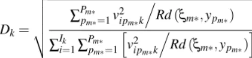
In comparison with FIMIX-PLS, PLS-TPM (Trinchera et al., 2006; Squillacciotti, 2007) uses a different statistical approach for response based segmentation issues. Considering that PLS path modeling aims at optimizing the models’ predictivity without requiring distri-butional assumptions, PLS-TPM has been designed for prediction oriented path model seg-mentation without including distributional assumptions on latent or manifest variables level. The assignment of the units to the latent classes is achieved throughout a unit-model dis-tance. The chosen distance is obtained as an extension of theDModYdistance used in PLS Regression (Tenenhaus and Esposito Vinzi, 2005; Bastien et al., 2005; Tenenhaus, 1998) and in PLS Typological Regression (PLS-TR; Esposito Vinzi et al., 2004). It is computed as follows:

Dk= ∑ Pm∗ pm∗=1v2ipm∗k Rd(ξm∗,ypm∗) ∑Ik i=1∑ Pm∗ pm∗=1 v2ipm∗k Rd(ξm∗,ypm∗) (12)

whereξm∗ is the target latent variable,v2ipm∗kis the residual of the redundancy model

(i.e., the regression of the final endogenous manifest variables over the exogenous target latent variables) andRd(ξm∗,ypm∗)represents the redundancy index for the target endoge-nous manifest variables for latent groupk. Until today, PLS-TPM has only been tested and implemented on models containing reflective latent variables, which is a frequent situation in applications. The distanceDkhas been developed for this kind of outer model. Ongoing

research extends the distance measure and thereby the methodology on the subject of its utilization in formative PLS path modeling.

Since the distance is computed in the endogenous manifest variables space, the obtained segmentation optimizes the prediction power of the local models in terms of the redundancy model. PLS-TPM performs an iterative algorithm to form the latent classes. The algorithm starts with a PLS path modeling analysis on all units. Based on the results of the global model, the residuals of the redundancy model are computed for each unit. Since the number of latent classes is not known a priori, a hierarchical classification is performed on these residuals. The dendrogram resulting from the ascendant hierarchical classification allows to choose the number of segments (K) corresponding to the optimal partition as well as their initial composition. Once the initial segments defined, the K local models are estimated. We thereby obtain the segment specific PLS path modeling results that allow computing the distances (Equation 12) of each unit from each local model.

Fig. 3 The PLS-TPM Algorithm begin

step 1:estimation of the global PLS path model

step 1.1:computation of the redundancy residuals of all units from the global model

step 1.2:ascendant hierarchical classification on the residuals computed at step 1.1

step 2:choice of the number of classes (K) according to the dendrogramme obtained at previous step

step 3:imputation of the units to each class according to the cluster analysis results; repeat do

begin

step 4:estimation of theKlocal models (one for each class)

step 5:computation of the distancesDkbetween each unit and each local model

step 6:assignment of each unit to the class corresponding to the closest local model end

until convergence

step 7:description of the obtained classes according to differences among the local models end

In every iteration, the distance of each unit from all local model is evaluated, and each unit is assigned to the closest local model with respect to the distanceDk. Modifications in

the class composition leads to reestimation of theKlocal models as well as the distances

Dkand reassignment of units. The stability of the composition of the classes or of the model

coefficients from one step to the other implies convergence of the algorithm. In other words, the algorithm converges when the results at theiiteration are the same (at the 2nd decimal figure) compared to those that have been generated in one of the previous iterations, or when the composition of the classes remains unchanged from one iteration to the other. The results

of the final local models are then compared with respect to the inner and outer coefficients. In PLS-TPM heterogeneity is not supposed to be limited to the inner model. Differently from FIMIX-PLS, outer coefficients are not static over the iterations but are reestimated at each step. Hence, PLS-TPM provides local models that are different not only in inner path coefficients but also in the outer relationships.

2.3 Response Based Unit Segmentation in PLS path modeling

PLS Typological Path modeling provides local models that are different with respect to both the inner and the outer models. Nonetheless, the segmentation of units is obtained only according to the inner model and to the target variable’s outer model. Moreover, PLS-TPM requires to identify a target latent variable among all the endogenous latent variables. For this reason, and in order to reach a segmentation of the units that takes into account the performance of both the inner and the outer models, a new response-based segmentation technique has been recently presented in the PLS path modeling framework: the REsponse-Based Units Segmentation (REBUS; Esposito Vinzi et al., 2007).

REBUS-PLS could be considered as a development of PLS-TPM aiming to overcome some of its major drawbacks: namely, the need to identify a target latent variable and the fact to provide a segmentation according to only the inner model.

The purpose of REBUS-PLS is to identify local models that are different as regard to both the inner and the outer models’ estimates and that fit better than the global model. That is why the observations are classified according to acloseness measure(CM) defined on the Goodness of Fit index structure (GoF; Tenenhaus et al., 2004).

GoF= ∑Qq=1∑ Pq p=1Cor2(xpq,ξq) ∑Q q=1Pq ×∑Mm=1R2(ξm,{ξj’s explaining ξm}) M (13)

whereQis the total number of latent variables (endogenous and exogenous ones),Mis the number of endogenous latent variables andPqis the number of manifest variables in the

q-th block.

As for theGoFindex (Equation 13), also thecloseness measureused in REBUS-PLS is formed by two different parts (Equation 14). The left-side term refers to the observations’ performance in the outer model, while the right-side term refers to the inner model. The basic idea is that if thei-th observation belongs to thek-th latent class, its performance in the local model estimated for thek-th latent class will be better than its performance in all the other local models. The performance of statistical units in the outer model is evaluated by the so called measurement or communality residuals (epqk), while their performance in

the inner model is assessed by taking into account the inner or structural residuals (fmk).

All the computed residuals are weighted according to quality indexes: the importance of residuals increases while the quality index decreases. That is why the communality index and theR2_{values are considered in theCM.}

CMik= ∑Q q=1∑ Pq p=1 e2ipqk/Com ξqk,xpq ∑I i∑Qq=1∑ Pq p=1 e2ipqk/Com(ξqk,xpq) (I−tk−1) ×∑Mm=1 f2 imk/R2(ξm,{ξj’s explaining ξm}) ∑I i∑Mm=1 fimk2 /R2 ξm,{ξj’s explaining ξm} (I−tk−1) (14)

whereeipqkis the measurement residual for thei-th observation in thek-th latent class,

corresponding to thep-th manifest variable in theq-th block, fimkis the structural residual

for thei-th observation in thek-th latent class, corresponding to them-th endogenous block,

Iis the total number of observations, andtkis the number of extracted components, since all

blocks are supposed to be reflective,tkwill always be equal to 1.

For each observation, one measurement residual is computed for each manifest variable and one structural residual is computed for each endogenous variable in the inner model. For a thorough description of the REBUS-PLS algorithm and the computation of the inner and the outer residuals, please refer to the original REBUS paper (Esposito Vinzi et al., 2007).

The choice of theCM as a criterion for assigning observations to latent classes has two major advantages. Firstly, unobserved heterogeneity can now be detected in both the measurement and the structural model. If two models show identical inner coefficients, but differ with respect to one or more outer weights in the exogenous blocks, REBUS-PLS is able to identify this source of heterogeneity differently from PLS-TPM and FIMIX-PLS. Moreover, since thecloseness measureis defined according to the structure of the GoF

index, the identified local models will show a higher value for both theGoF and theR2

indices.

Similarly to PLS-TPM and FIMIX-PLS, the REBUS-PLS algorithm starts by perform-ing a PLS path model analysis on the whole set of observations. Once the global model estimated, inner and outer residuals are computed. If no a priori information is available on the number of latent classes, as it is often the case, a hierarchical cluster analysis is per-formed on the computed residuals. The number of latent classes to take into account, as well as the initial composition of the latent classes, is obtained by looking at the dendogramme. A local model is then estimated for each identified latent class. For each observation, a close-ness measure from each local model is computed according to (Equation 14). Observations are then allocated to the closest local model, i.e. to the local model for which they show the smallestCMvalue. Changes in the latent classes composition lead to a new estimation of the local models and to a new computation ofCMs.

The algorithm stops when less than 0.5% of units change class membership from an iteration to another. The threshold value of the 0.5% is a rule of thumb obtained according to simulation and practical applications of the REBUS-PLS algorithm in order to take into account the so called boundary-observations. If users force the algorithm to go beyond this threshols, the algorithm keeps providing the same results in terms of classes composition and local models’ estimates in the successive steps.

Ex-post analysis could be performed in order to identify external (concomitant) vari-ables that characterize the latent classes identified by REBUS-PLS. It is important to un-derline that local models of REBUS-PLS differ with respect to both the inner and the outer estimates. Moreover, external information is used only to describe the latent classes iden-tified by REBUS-PLS: the latent classes’ composition is obtained according to inner and outer models’ residuals.

3 Design of the Numerical Example and Data Simulation

A key area for identifying and forming segments in social sciences is related to the specific behavior of certain groups of persons. Although the naming of latent variables is a trivial matter for numerical examples using simulated data, this study focuses on the area of cus-tomer satisfaction (Fornell et al., 1996) as well as segmentation of markets and consumers (Wedel and DeSarbo, 2002). We thereby identify heterogeneity and treat it by segmentation

Fig. 4 The REBUS-PLS Algorithm begin

step 1:estimation of the global PLS path model

step 1.1:computation of the inner and outer residuals of all observations from the global model

step 1.2:ascendant hierarchical classification on the residuals computed at step 1.1

step 2:choice of the number of classes (K) according to the dendrogramme obtained at previous step

step 3:imputation of the observations to each class according to the cluster analysis results repeat do

begin

step 4:estimation of theKlocal models (one for each class)

step 5:computation of thecloseness measure CM_kbetween each observation and each local model

step 6:assignment of each observation to the class corresponding to the closest local model end

until convergence

step 7:description of the obtained classes according to differences among the local models end

as means of presenting the general effectiveness of FIMIX-PLS and PLS-TPM for path mod-eling. This kind of example allows us to better illustrate the motivation and consequences of this study that are for the most part transferable to other research disciplines in social sciences.

Customer satisfaction has become a fundamental and well documented construct in busi-ness research. It is critical to demand and to any corporation’s success given its importance and established relation to customer retention and corporate profitability (Anderson et al., 1994). Although it is often acknowledged that truly homogeneous segments of consumers do not exist, studies even report unobserved customer heterogeneity within a given product or service class (Wu and Desarbo, 2005). Forming groups of consumers that are homogeneous in terms of the benefits they seek or their response to marketing programs (e.g. product of-fering, price discounts) is therefore a key element for marketers to establish and improve their targeted marketing strategies (Wedel and Kamakura, 2000).

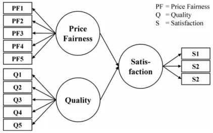
In terms of heterogeneity in the inner path model, it might be desirable to identify and describe price sensitive consumers or those requiring price fairness (Xia et al., 2004) and consumers who have the strongest preference for another particular product attribute (Al-lenby et al., 1998), e.g. quality. Thus, the path model for our numerical examples (Figure 5) has one latent endogenous variable,Customer Satisfaction, and two latent exogenous vari-ables,Price FairnessandQuality, in the inner model (Jedidi et al., 1997). The experimental sets of data consist of two segments with the following characteristics: (a) Segment 1 (price fairness seeking customers) is characterized by a strong relationship betweenPrice Fairness

andCustomer Satisfactionand a weak relationship betweenQualityandCustomer

Satisfac-tion; (b) Segment 2 (quality oriented customers) is characterized by a strong relationship betweenQualityandCustomer Satisfactionand a weak relationship betweenPrice Fairness

andCustomer Satisfaction.

Each latent exogenous variable (Price FairnessandQuality) has five manifest variables (reflective mode), and the latent endogenous variable (Customer Satisfaction) is measured by three indicators (reflective mode). However, it is not relevant for this study to include an additional level of complexity by exemplifying path model details regarding the manifest variables and the theoretical reasoning for choosing reflective instead of formative measure-ment models (c.f. Bagozzi and Edwards, 2005). PLS-TPM has been established for path models with reflective blocks and, thus, our analysis is limited to that kind of measurement model.

Fig. 5 PLS Path Model for Data Simulation

This study intentionally uses a clear cut example of a marketing related path model for data simulation purposes. We principally follow the data generation procedure that Chin et al. (2003) use for PLS path modeling. Data for each segment is first generated for the latent variables according to the relationships specified in inner path model and then data is generated for the observed variables from the latent variables in the model. This approach allows to generate data with distributional characteristics imposed by the model (Chin et al., 2003) and is consistent with the functionalities available in the SEPATH module of the software application STATISTICA 7.1 (StatSoft, Inc., 2005). Data simulation for the group of price fairness seeking consumers involves a strong relationship of 0.9 betweenPrice

Fairnessand Customer Satisfactionand a week relationship of 0.1 betweenQualityand

Customer Satisfactionin the inner path model (Segment 1). Another group of data reflects

the characteristics of the quality oriented consumers (Segment 2). To start with, we simulate normal data of 100 cases per segment. Thus, data on the aggregate level for the numerical examples includes 200 cases.

An evaluation of FIMIX-PLS and PLS-TPM capabilities requires alterations of segment sizes and data distribution. Keeping the total number of cases at 200, we also simulate data for different segment proprtions, namely 0.6 to 0.4, 0.7 to 0.3 and 0.8 to 0.2. Thereby, this study exhibits whether the model based segmentation techniques for PLS correctly identify the groups when their sizes are systematically changed. Moreover, this analysis includes data that is nonnormal for the three cases of (a) skewness, (b) kurtosis and (c) both, skew-ness and kurtosis. Skewskew-ness has a value 0.85 and kurtosis has a value of 2.0. In accordance with other studies (c.f. Boomsma and Hoogland, 2001), the selected value of skewness and kurtosis are at moderate levels. Vale and Maurelli (1983) extended the Fleishman approach to generate multivariate nonnormal random numbers. This procedure, as it is implemented in the STATISTICA software application, fits our nonnormal data generation purposes espe-cially since control of specified nonnormal distributions in latent variables is not of interest to us (Reinartz et al., 2002).

In total, the analysis involves 16 marketing related numerical examples on different sets of simulated data. Each set includes computation of PLS path modeling results for (a) the aggregate data level (global model) and (b) each group of simulated data (group

models) as well as the class or local model solutions for (c) FIMIX-PLS employing the SmartPLS 2.0 (Ringle et al., 2005) software application and (d) PLS-TPM using a SAS macro implementation (Trinchera et al., 2006). The results of the global model exhibit the requirement for addressing heterogeneity of inner path model estimates. A comparison of the outcomes in the group and local models estimates facilitates an assessment of FIMIX-PLS and FIMIX-PLS-TPM. The group model estimates for the two high and low inner path model coefficients as well asR2_{of the latent endogenous variables satisfaction are benchmarks for}

both model based segmentation techniques. The rate of correctly assigned cases is another performance indicator. In order to evaluate that rate for FIMIX-PLS, data is classified by their probabilities of membership into the two final groups. TheEN(Hahn et al., 2002) and theGoF(Tenenhaus et al., 2005) are specific evaluation criteria for each methodology that we include in our analysis. Evaluation of class separation in FIMIX-PLS uses theEN. This criterion requires probabilities of membershipPikand, thus, is inappropriate for PLS-TPM.

On the other hand, theGoF is a global evaluation criterion for model quality, which takes both the redundancy and the communality model into account. FIMIX-PLS cannot estimate class specific out relationships that are required for computing theGoF.

The design of this study allows us to present three kinds of analyses. First, we reveal the requirement and the potentials of FIMIX-PLS and PLS-TPM to detect (unobserved) hetero-geneity in the inner path model relationships for different sets of simulated data. Second, the numerical examples give evidence how both methodologies perform in situations of unbal-anced group sizes. Third, this study exhibits the capabilities of FIMIX-PLS and PLS-TPM to uncover the segments when data is nonnormal.

4 Simulation Study on Partial Least Squares Path Model Based Identification of Heterogeneity and Segmentation

4.1 Results on the Aggregate Data Level

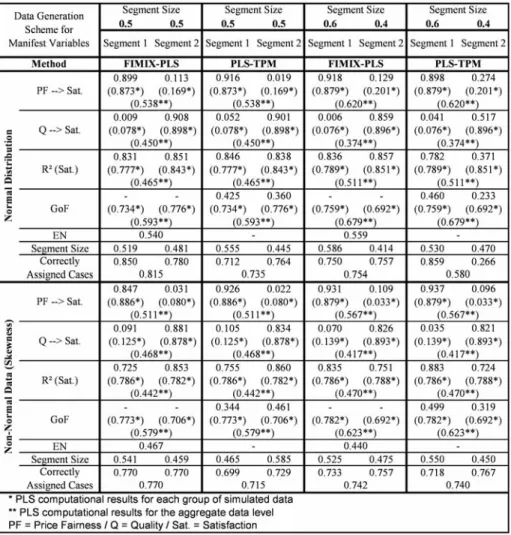
Before we analyze the results of model based segmentation for FIMIX-PLS and, thereafter, for PLS-TPM, it is important to illustrate the requirement for these kinds of analyses. The PLS path modeling results on the aggregate data level (Figure 6 to Figure 9) are significantly different compared with the segment specific computations for each a priori simulated group of data. In these numerical examples, estimates for the overall set of data are close to the weighted average of group specific coefficients. As a consequence, the PLS path modeling results are ambiguous when heterogeneity is not accounted for, especially when distinctive groups have about the same size. For instance, in the numerical example for the 0.5 to 0.5 segment sizes case, the two inner relationships of about 0.9 and 0.1 for one group and vice versa for the other group of simulated data turn out to have a value on the aggregate data level between 0.450 and 0.550 for both relationships. Moreover,R2_{is significantly lower}

than for the PLS estimations for each group of data.

If heterogeneity is not identified by the researcher, the effects of Price Fairnessand

QualityonSatisfactionseem to be equally important, at least in the numerical examples

with equal segments sizes. As a consequence of these PLS path modeling results, marketers may focus on the areas ofPrice FairnessandQualityat the same time for all consumers. Uncovering heterogeneity the inner path model relationships and forming distinctive groups of price fairness seeking and quality oriented customers allows marketers to develop better targeted and more effective business strategies. However, the requirement for model based

Fig. 6 FIMIX-PLS and PLS-TPM Results for Simulated Data (Part A)

segmentation decreases when on segment dominates the other and thereby the path model estimates on the aggregate data level.

4.2 Result for the Finite Mixture Partial Least Squares Approach

The simulation study reveals that the FIMIX-PLS methodology is capable to reliably un-cover heterogeneity in all 16 examples under evaluation (Figure 6 to Figure 9). This finding is based on the FIMIX-PLS results for mixing proportions, segments specific path coef-ficients, and theR2 ofSatisfaction. Most important, the FIMIX-PLS mixing proportions, which are computed including the probabilities of membership of each case (Figure 2), and inner path model coefficients for each class are very close to the pre-determined segment sizes and relationships in all numerical examples. Moreover, with respect to the assumption that FIMIX-PLS aims at separating segment specific distributional functions with

condi-tional multivariate normal densities (Hahn et al., 2002), it is essential to note that the iden-tification of segments is very robust regarding violations of the multivariate distributional assumption. FIMIX-PLS appropriately uncovers the two a priori formed segments even in situations when data is extremely nonnormal (the case of skewness and kurtosis).

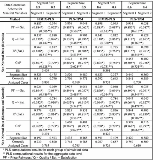
Fig. 7 FIMIX-PLS and PLS-TPM Results for Simulated Data (Part B)

This study on simulated data does not include an explanatory variable for final seg-mentation according to stage two of a comprehensive FIMIX-PLS analysis (Figure 1). As an alternative, we use thePikresults to assign each case to one of the two segments and,

thereby, to assess their correct assignment in each numerical example. The overall rate of correctly assigned cases ranges from 0.726 to 0.905. This is a sufficiently high level to pos-itively evaluate the capabilities of FIMIX-PLS considering that data simulation includes a certain number of cases that fit well in one and in the other group and represent noisy data in the intersection of both generated segments. TheENcomputation includes the probabilities

of membership to indicate how well classes are separable. A value ofENabove 0.5 in the different sets of normal data with altered segments sizes gives evidence that the observations have relatively highPikand, thus, the data is well separable into two groups (Ringle et al.,

2007). The decline ofENbelow 0.5 in numerical examples for nonnormal data reveals that classification becomes more ambiguous in terms ofPik. A comparison of the three cases

of nonnormal data discloses that ”skewness” provides better results than ”kurtosis” regard-ing the rate of correctly assigned cases while ”kurtosis” performs better than ”skewness” in terms ofEN. The combination of kurtosis and skewness joins both weak effects.

Regardless whether data is normal or nonnormal, in the numerical examples for the 0.5 to 0.5 segment sizes, FIMIX-PLS provides class specific path coefficients that are compa-rable to those PLS estimates for each a priori formed segment and an in average increased

R2. However, the methodology has a tendency to produce more distinctive segment specific path coefficients and a higherR2_{outcome for one segment when the segment sizes are}

sys-tematically changed. This tendency towards capitalizing on certain segments is determined by the FIMIX-PLS methodology. In particular, the most important determinants are (a) the segment sizes as well as, (b) the heterogeneity and, thus, the distinctiveness of data for sep-aration regarding the path coefficients, and (c) the level ofR2in the PLS estimates for each group of simulated data. The more those criteria direct the algorithm towards a particular segment, the higher are its FIMIX-PLS differences of segment specific path coefficients and the increase ofR2_{compared to the results for each a priori formed segment.}

As a consequence, the rate of correctly assigned cases increases for the larger segment while that for the smaller segments declines resulting in an enhanced overall appropriateness of assignment in this study. We finally find that in the examples of normal and kurtic dataPik

is relatively high when the cases are correctly clustered. Otherwise,Pikis close to 0.5 in these

numerical examples for two classes. Accordingly,ENsystematically rises when the segment sizes further diverge considering the methodology’s tendency to increase the percentage of correctly assigned cases for the larger segment. However, this kind of outcome does not hold when skewness is involved. FIMIX-PLS computations become more fuzzy regarding

Pikand, thus,ENis at lower levels. Moreover, increases (decreases) of the size of the smaller

(larger) segment results in a cutback of the effect that the cases of the larger segment improve in their rate of correct assignment at cost of the smaller segment.

These finding support the reliability and robustness of FIMIX-PLS. In situations when nonnormality of data becomes an issue, the researcher must carefully consider the effects of kurtosis and skewness on the FIMIX-PLS results. The reliability of results depends on the degree of inner path model heterogeneity as well as the nonnormality of data. Our study gives evidence that FIMIX-PLS clearly indicates potential problems of unobserved hetero-geneity even in extreme data constellation.

4.3 Segmentation Using Partial Least Squares Typological Path Modeling

In all data sets PLS-TPM unfolds two classes: one shows a high structural relationship from

Price FairnesstoSatisfactionand a non significant relationship betweenQualityand

Satis-factionwhile the other one shows exactly the opposite characteristics. The original

simula-tion scheme is thus respected. All local models lead to a better model performance in terms ofR2_{compared to the global model. However, the final local models results show globally}

lower values for theGoF. This is due to the chosen distance measure, which optimizes the local redundancy models’ predictivity (R2_{) and does not take the exogenous variables’ local}

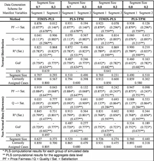
Fig. 8 FIMIX-PLS and PLS-TPM Results for Simulated Data (Part C)

models into account. A generalization of the distance measure in order to also account for exogenous blocks’ communality is subject of ongoing research.

In data sets where groups are mixed in equal proportions, well classified rates are in all cases higher than 0.72. The worst results are obtained for the data generated with skewness, and the best result for the data characterized by kurtosis. In the data sets with groups showing different mixing proportions, the well classified rates for all data sets become on the whole lower, especially when the size of one group becomes very small compared to the other. In such situations, one of the two groups has a far higher weight in the definition of the structural coefficients of the global model instead of having a starting sample where quality oriented and price fairness seeking customers are mixed in equal proportions and, hence, a global model resulting as an ”average” of the two groups. In other words, the global model is already price fairness seeking, making it harder to ”isolate” the units with a different

behavior. This finding is substantiated by the results for constellations where well classified rates are generally higher in the largest group.

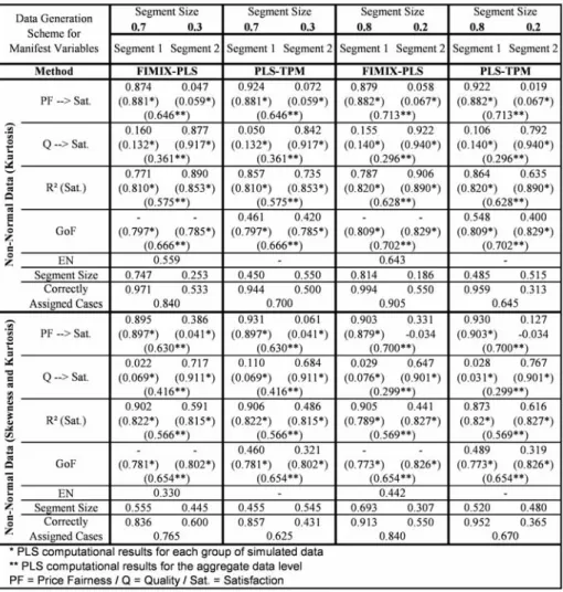
Fig. 9 FIMIX-PLS and PLS-TPM Results for Simulated Data (Part D)

The PLS-TPM performs very efficiently in the numerical examples under evaluation. The highest number of iterations (19) before convergence was required for data generated with high skewness. In all three remaining data sets, less than 14 iterations led to conver-gence.

4.4 Comparison of Results

FIMIX-PLS and PLS-TPM are the first PLS related statistical approaches for model based identification of heterogeneity. Both methodologies are able to detect the two latent classes

in all numerical examples using different sets of simulated data. However, their statistical foundations are diametrical unalike. Our primary analysis and comparison reveals certain characteristics that are important for researchers and practitioners when evaluating PLS path modeling results by employing FIMIX-PLS and PLS-TPM. In general, advantages of one approach are disadvantages of the other.

FIMIX-PLS uses underlying distributional assumptions to form the latent classes. As a result, the procedure provides the probabilities of membership for each case to belong the

klatent class. Computations of all other FIMIX-PLS results are based onPik. Even though

exhibiting a strong robustness, nonnormality of data negatively affects the method’s perfor-mance. In contrast, PLS-TPM estimates the model parameters for each segment in every iteration and units are unambiguously assigned to the closest local model regarding the dis-tance defined in Equation 12. The researcher or practitioners does not obtain Pik related

results but the final separation intoKdistinctive (non overlapping) sets of data and their seg-ment specific PLS path model estimates. PLS-TPM is a distribution-free method. Results are on similar levels regardless whether data is normal or nonnormal. However, PLS-TPM uses a distance measure that exhibits the tendency to form groups of equal size. Uneven segment sizes have a negative effect on the performance of this approach. In contrast, FIMIX-PLS estimations for each class and segments sizes usually meet the expectations regarding the a priori formed groups of data in the numerical examples. However, certain determinants, e.g. unbalanced segments sizes, cause a tendency to prefer one segment above the other. The FIMIX-PLS results for the larger class turn out to be slightly better in this study. This behavior also holds true in PLS-TPM.

Both FIMIX-PLS and PLS-TPM account for heterogeneity in the inner path model re-lationships. It is desirable that model based segmentation also identifies segment specific differences in the formative outer model relationships. This mode of PLS estimations is of high relevance in analyses, for example, on success factors in the strategic management or marketing disciplines. PLS-TPM is a key development into that direction. The methodology uses a distance measure that focuses on the redundancy model, reestimates the entire model in each iteration and, thus, considers the specific outer relationships of each local model when forming segments. But in the current state of development, the methodology is only applicable to path models involving reflective measurement models. Future research on the distance measure as well as on the optimization criterion and its behavior must exploit the potential capabilities of PLS-TPM to accomplish segmentation for all path model relation-ships. On the contrary, the FIMIX-PLS optimization criterion is definite and only aims at the inner model estimates. The algorithm uses static latent variable scores as input for la-tent class segmentation (Figure 1). As a consequence, the methodology has no capabilities to explicitly account for heterogeneity in outer relationships. This is a drawback in prac-tical applications but allows for general applicability to PLS path modeling. FIMIX-PLS reliably identifies heterogeneity in inner path model relationships regardless whether outer measurement model operationalization is in the formative or reflective mode (Ringle et al., 2007).

5 Conclusion and Future Research

The numerical examples on customer satisfaction demonstrate that interpretation of PLS path modeling results on the aggregate data level is misleading whenever they involve het-erogeneity inner model estimates. Our study gives evidence that FIMIX-PLS and PLS-TPM reliably identify this kind of heterogeneity and guide separation of the two a priori created

groups of price fairness seeking and quality oriented customers. The model based segmen-tation techniques provide additional analytical findings where conventional clustering meth-ods fail. Researchers and practitioners can exploit these PLS model based segmentation techniques to assure that results on the aggregate data level are not affected by unobserved heterogeneity in the inner path model estimates. Otherwise, FIMIX-PLS and PLS-TPM in-dicate how to treat that problem by forming groups of data. A multigroup PLS path analysis on the finally established segments (Chin and Dibbern, 2007) gives evidence if segment specific estimates are significantly different. In this case, researchers or practitioners obtain supplementary analytical results to single out their conclusions, in example, to form business strategies that effectively target certain customer segments. We believe that FIMIX-PLS and PLS-TPM are key extensions of PLS path modeling and will become a standard procedures for evaluating results.

Our initial assessment and comparison of both methodologies reveals certain strengths of each approach that are by some extent weaknesses of the other. We find that FIMIX-PLS is a generally applicable method for PLS path modeling, accurately identifies the class sizes and determines their distinctiveness in terms ofEN. In contrast, we conclude that PLS-TPM does not require distributional assumptions, dynamically updates group specific PLS esti-mations and, thereby, provides a final assignment of observations to segments that is not based on probabilities of membership. In view of these different characteristics, a combined application of both methodologies in PLS path modeling is most effective to researchers and practitioners. In the first stage, FIMIX-PLS indicates whether heterogeneity in inner path model estimates represents a problem for the PLS analysis by rendering an appropriate number of groups, their sizes, and how well they can be separated regardingENas well as segment specific inner model estimates. In the next stage, PLS-TPM provides segmentation and PLS estimations for each group of data. We finally conclude that the PLS-TPM method-ology better fits the statistical characteristics of PLS path modeling and has more potentials for extensions to improve model based segmentation.

The present work is an initial contribution on the subject of segmentation techniques in PLS path modeling. In this sense, many aspects of the methodologies require further in-vestigations. Future research on PLS-TPM must extend the methodology on formative mea-surement models and, thereby, address its general applicability to PLS path modeling. More specifically, the distance measure that determines the optimization criterion of classification performed through PLS-TPM and the convergence properties of the PLS-TPM algorithm requires further analyses. An additional evaluation criterion, similar toENfor FIMIX-PLS, must indicate the distinctiveness of distances for the assignment of cases to the final local models. Future research on FIMIX-PLS must address known problems regarding, for ex-ample, local optimum solutions or non-interpretable FIMIX-PLS estimates (Ringle et al., 2007). A critical issue of both approaches is the identification of an explanatory variable that allows the kind of segmentation as indicated by FIMIX-PLS or PLS-TPM. The devel-opment of appropriate methodologies is essential to complement model based segmentation. Moreover, a first numerical assessment and comparison of both approaches cannot state the general validity of our conclusions. Our analysis is limited to one kind of path model, two segments and a single set of data for each numerical example. Future research must present extensive simulation studies with experimental data and a broad use of empirical data to assess FIMIX-PLS and PLS-TPM capabilities for a variety of data and path model constel-lations.

References

Allenby, G. M., Arora, N., Ginter, J. L., 1998. On the heterogeneity of demand. Journal of Marketing Research 35 (3), 384–389.

Anderson, E. W., Fornell, C., Lehmann, D. R., 1994. Customer satisfaction, market share, and profitability: findings from Sweden. Journal of Marketing 58 (3), 53–66.

Bagozzi, R. P., Edwards, J. R., 2005. On the nature and direction of relationships between constructs and measures. Psychological Methods 2 (5), 155–174.

Barnard, G. A., 1958. Studies in the history of probability and statistics: IX. Thomas Bayes’s essay towards solving a problem in the doctrine of chances. Biometrika 45 (3/4), 293–315. Bastien, P., Tenenhaus, M., Esposito Vinzi, V., 2005. PLS generalised linear regression.

Computational Statistics & Data Analysis 48 (1), 17–46.

Boomsma, A., Hoogland, J. J., 2001. The robustness of LISREL modeling revisited. In: Cudeck, R., du Toit, S., S¨orbom, D. (Eds.), Structural Equation Modeling: Present and Future. Scientific Software International, Chicago, pp. 139–168.

Chin, W. W., 1998. Issues and opinion on structural equation modeling. MIS Quarterly 22 (1), XII–XVI.

Chin, W. W., Dibbern, J., 2007. A permutation based procedure for multi-group PLS anal-ysis: Results of tests of differences on simulated data and a cross cultural analysis of the sourcing of information system services between Germany and the USA. In: Esposito Vinzi, V., Chin, W. W., Henseler, J., Wang, H. (Eds.), Handbook of Partial Least Squares: Concepts, Methods and Applications in Marketing and Related Fields - Forthcoming. Springer, Berlin et al.

Chin, W. W., Marcolin, B. L., Newsted, P. N., 2003. A partial least squares approach for measuring interaction effects: Results from a Monte Carlo simulation study and an elec-tronic mail emotion/adoption study. Information Systems Research 14 (2), 189–217. Diamantopoulos, A., Winklhofer, H., 2001. Index construction with formative indicators: an

alternative to scale development. Journal of Marketing Research 38 (2), 269–277. Esposito Vinzi, V., Lauro, C., Amato, S., 2004. PLS typological regression: Algorithmic,

classification and validation issues. In: Vichi, M., Monari, P., Mignani, S., Montanari, A. (Eds.), New Developments in Classification and Data Analysis. Springer, Berlin et al., pp. 133–140.

Esposito Vinzi, V., Trinchera, L., Squillacciotti, S., Tenenhaus, M., 2007. REBUS-PLS: A response - based procedure for detecting unit segments in pls path modeling. submitted to Applied Stochastic Models in Business and Industry (ASMBI).

Fornell, C., Bookstein, F. L., 1982. Two structural equation models: LISREL and PLS ap-plied to consumer exit-voice theory. Journal of Marketing Research 19 (4), 440–452. Fornell, C., Johnson, M. D., Anderson, E. W., Jaesung, C., Bryant, B. E., 1996. The

Amer-ican customer satisfaction index: Nature, purpose, and findings. Journal of Marketing 60 (4), 7–18.

Fornell, C., Lorange, P., Roos, J., 1990. The cooperative venture formation process: A latent variable structural modeling approach. Management Science 36 (10), 1246–1255. Fornell, C., Robinson, W. T., Wernerfelt, B., 1985. Consumption experience and sales

pro-motion expenditure. Management Science 31 (9), 1084–1105.

Gerbing, D. W., Anderson, J. C., 1988. An updated paradigm for scale development in-corporating unidimensionality and its assessment. Journal of Marketing Research 25 (2), 186–192.

Gray, P. H., Meister, D. B., 2004. Knowledge sourcing effectiveness. Management Science 50 (6), 821–834.

Hahn, C., Johnson, M. D., Herrmann, A., Huber, F., 2002. Capturing customer heterogeneity using a finite mixture PLS approach. Schmalenbach Business Review 54 (3), 243–269. Henseler, J., Fassott, G., 2007. Testing moderating effects in PLS path models: An

illus-tration of available procedures. In: Esposito Vinzi, V., Chin, W. W., Henseler, J., Wang, H. (Eds.), Handbook of Partial Least Squares: Concepts, Methods and Applications in Marketing and Related Fields - Forthcoming. Springer, Berlin et al.

Jedidi, K., Jagpal, H. S., DeSarbo, W. S., 1997. Finite-mixture structural equation models for response-based segmentation and unobserved heterogeneity. Marketing Science 16 (1), 39–59.

J¨oreskog, K. G., 1978. Structural analysis of covariance and correlation matrices. Psychome-trika 43 (4), 443–477.

Lohm¨oller, J.-B., 1989. Latent Variable Path Modeling with Partial Least Squares. Physica, Heidelberg.

Marcoulides, G. A., Saunders, C., 2006. PLS: A silver bullet? MIS Quarterly 30 (2), iii–ix. Ramaswamy, V., DeSarbo, W. S., Reibstein, D. J., Robinson, W. T., 1993. An empirical

pooling approach for estimating marketing mix elasticities with PIMS data. Marketing Science 12 (1), 103–124.

Reinartz, W. J., Echambadi, R., Chin, W. W., 2002. Generating non-normal data for sim-ulation of structural equation models using mattson’s method. Multivariate Behavioral Research 37 (2), 227–244.

Rigdon, E. E., 1998. Structural equation modeling. In: Marcoulides, G. A. (Ed.), Modern Methods for Business Research. Erlbaum, Mahwah, pp. 251–294.

Ringle, C. M., 2006. Segmentation for path models and unobserved heterogeneity: The finite mixture partial least squares approach. Research Papers on Marketing and Retailing No. 35, Hamburg.

Ringle, C. M., Wende, S., Will, A., 2005. SmartPLS 2.0. http://www.smartpls.de.

Ringle, C. M., Wende, S., Will, A., 2007. Finite mixture partial least squares analysis: Methodology and numerical examples. In: Esposito Vinzi, V., Chin, W. W., Henseler, J., Wang, H. (Eds.), Handbook of Partial Least Squares: Concepts, Methods and Applica-tions in Marketing and Related Fields - Forthcoming. Springer, Berlin et al.

Squillacciotti, S., 2007. Prediction-oriented classification in PLS path modeling. In: Es-posito Vinzi, V., Chin, W. W., Henseler, J., Wang, H. (Eds.), Handbook of Partial Least Squares: Concepts, Methods and Applications in Marketing and Related Fields - Forth-coming. Springer, Berlin et al.

StatSoft, Inc., 2005. STATISTICA for Windows Version 7.1. http://www.statsoft.com. Tenenhaus, M., 1998. La r´egression PLS. Technip, Paris.

Tenenhaus, M., Amato, S., Esposito Vinzi, V., 2004. A global goodness-of-fit index for pls structural equation modelling. In: Proceedings of the XLII SIS Scientific Meet-ing,Contributed Papers. CLEUP, Padova, pp. 739–742.

Tenenhaus, M., Esposito Vinzi, V., 2005. PLS regression, PLS path modeling and gen-eralized Procrustean analysis: a combined approach for multiblock analysis. Journal of Chemometrics 19 (3), 145–153.

Tenenhaus, M., Esposito Vinzi, V., Chatelin, Y.-M., Lauro, C., 2005. PLS path modeling. Computational Statistics & Data Analysis 48 (1), 159–205.

Trinchera, L., Squillacciotti, S., Esposito Vinzi, V., 2006. PLS typological path modeling: A model-based approach to classification. In: Esposito Vinzi, V., Lauro, C., Braverman, A., Schimek, M. G., Kiers, H. A. (Eds.), Electronic Proceedings of Knowledge Extraction and Modeling Conference.