A Discriminative Learning Model for Coordinate Conjunctions
Masashi Shimbo∗
Graduate School of Information Science Nara Institute of Science and Technology
Ikoma, Nara 630-0192, Japan [email protected]
Kazuo Hara∗
Graduate School of Information Science Nara Institute of Science and Technology
Ikoma, Nara 630-0192, Japan [email protected]
Abstract
We propose a sequence-alignment based method for detecting and disambiguating co-ordinate conjunctions. In this method, av-eraged perceptron learning is used to adapt the substitution matrix to the training data drawn from the target language and domain. To reduce the cost of training data con-struction, our method accepts training exam-ples in which complete word-by-word align-ment labels are missing, but instead only the boundaries of coordinated conjuncts are marked. We report promising empirical re-sults in detecting and disambiguating coor-dinated noun phrases in the GENIA corpus, despite a relatively small number of train-ing examples and minimal features are em-ployed.
1 Introduction
Coordination, along with prepositional phrase at-tachment, is a major source of syntactic ambiguity in natural language. Although only a small number of previous studies in natural language processing have dealt with coordinations, this does not mean disambiguating coordinations is easy and negligible; it still remains one of the difficulties for state-of-the-art parsers. in Charniak and Johnson’s recent work (Charniak and Johnson, 2005), for instance, two of the features incorporated in their parse reranker are aimed specifically at resolving coordination ambi-guities.
Previous work on coordinations includes (Agar-wal and Boggess, 1992; Chantree et al., 2005;
Kuro-∗Equal contribution.
hashi and Nagao, 1994; Nakov and Hearst, 2005; Okumura and Muraki, 1994; Resnik, 1999). Ear-lier studies (Agarwal and Boggess, 1992; Okumura and Muraki, 1994) attempted to find heuristic rules to disambiguate coordinations. More recent re-search are concerned with capturing structural sim-ilarity between conjuncts using thesauri and cor-pora (Chantree et al., 2005), or web-based statistics (Nakov and Hearst, 2005).
We identify three problems associated with the previous work.
1. Most of these studies evaluate the proposed heuristics against restricted forms of conjunc-tions. In some cases, they only deal with co-ordinations with exactly two conjuncts, leaving the generality of these heuristics unclear.
2. Most of these studies assume that the bound-aries of coordinations are known in advance, which, in our opinion, is impractical.
3. The proposed heuristics and statistics capture many different aspects of coordination. How-ever, it is not clear how they interact and how they can be combined.
To address these problems, we propose a new framework for detecting and disambiguating coor-dinate conjunctions. Being a discriminative learning model, it can incorporate a large number of overlap-ping features encoding various heuristics for coordi-nation disambiguation. It thus provides a test bed for examining combined use of the proposed heuristics as well as new ones. As the weight on each feature is automatically tuned on the training data, assessing these weights allows us to evaluate the relative merit of individual features.
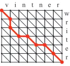
w r i t e r n t n e r i
[image:2.612.151.220.60.125.2]v
Figure 1: An alignment between ’writer’ and ’vint-ner,’ represented as a path in an edit graph
Our learning model is also designed to admit ex-amples in which only the boundaries of coordinated conjuncts are marked, to reduce the cost of training data annotation.
The state space of our model resembles that of Kurohashi and Nagao’s Japanese coordination de-tection method (Kurohashi and Nagao, 1994). How-ever, they considered only the decoding of coordi-nated phrases and did not address automatic param-eter tuning.
2 Coordination disambiguation as sequence alignment
It is widely acknowledged that coordinate conjunc-tions often consist of two or more conjuncts having similar syntactic constructs. Our coordination detec-tion model also follows this observadetec-tion. To detect such similar constructs, we use the sequence align-ment technique (Gusfield, 1997).
2.1 Sequence alignment
Sequence alignment is defined in terms of transfor-mation of one sequence (string) into another through analignment, or a series of edit operations. Each of the edit operations has an associated cost, and the cost of an alignment is defined as the total cost of edit operations involved in the alignment. The min-imum cost alignment can be computed by dynamic programming in a state space called anedit graph, such as illustrated in Figure 1. In this graph, a com-plete path starting from the upper-left initial vertex and arriving at the lower-right terminal vertex con-stitutes a global alignment. Likewise, a partial path corresponds to a local alignment.
Sequence alignment can also be formulated with thescoresof edit operations instead of theircosts. In this case, the sequence alignment problem is that of finding a series of edit operations with the maximum
score.
2.2 Edit graph for coordinate conjunctions
A fundamental difference between biological local sequence alignment and coordination detection is that the former deals with finding local homologies between two (or more) distinct sequences, whereas coordination detection is concerned with local simi-larities within a single sentence.
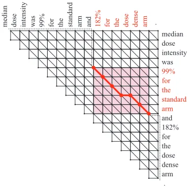
The maximal local alignment between two iden-tical sequences is a trivial (global) alignment of identity transformation (the diagonal path in an edit graph). Coordination detection thus reduces to find-ingoff-diagonal partial paths with the highest sim-ilarity score. Such paths never cross the diagonal, and we can limit our search space to the upper trian-gular part of the edit graph, as illustrated in Figure 2.
3 Automatic parameter tuning
Given a suitable substitution matrix, i.e., function from edit operations to scores, it is straightforward to find optimal alignments, or coordinate conjunc-tions in our task, by running the Viterbi algorithm in an edit graph.
In computational biology, there exist established substitution matrices (e.g., PAM and BLOSUM) built on a generative model of mutations and their associated probabilities.
Such convenient substitution matrices do not ex-ist for coordination detection. Moreover, optimal score functions are likely to vary from one domain (or language) to another. Instead of designing a specific function for a single domain, we propose a general discriminative learning model in which the score function is a linear function of thefeatures as-signed to vertices and edges in the state space, and the weight of the features are automatically tuned for given gold standard data (training examples) drawn from the application domain. Designing heuristic rules for coordination detection, such as those pro-posed in previous studies, translates to the design of suitable features in our model.
median dose intensity was
99% for standard
arm 182%
the dose
arm
and
for
the
dense
[image:3.612.344.507.57.100.2]. median dose intensity was 99% for the standard arm and 182% for the dose dense arm .
Figure 2: An edit graph for coordinate detection
1. Collins’s method, like the linear-chain condi-tional random fields (CRFs) (Lafferty et al., 2001; Sha and Pereira, 2003), seeks for a com-plete path from the initial vertex to the terminal using the Viterbi algorithm. In an edit graph, on the other hand, coordinations are represented by partial paths. And we somehow need to complement the partial path to make a com-plete path.
2. A substitution matrix, which defines the score of edit operations, can be represented as a func-tion of features defined on edges. But to deal with complex coordinations, a more expressive score function is sometimes desirable, so that scores can be computed not only on the basis of a single edit operation, but also on consecutive edit operations. Edit graphs are not designed to accommodate features for such a higher-order interaction of edit operations.
To reconcile these incompatibilities, we derive a more finer-grained model from the original edit graph. In presenting the description of our model be-low, we reserve the terminology ‘vertex’ and ‘edge’ for the original edit graph, and use ‘node’ and ‘arc’ for our new model, to avoid confusion.
3.1 State space for learning coordinate
conjunctions
The new model is also based on the edit graph. In this model, we create a node for each triple(v,p,e),
(a) (b) (c) (d) (e)
Figure 3: Five node types created for a vertex in an edit graph: (a)Inside Delete, (b)Inside Insert, (c) In-side Substitute, (d)Outside Delete, and (e)Outside Insert.
[image:3.612.93.278.59.244.2](a) (b)
Figure 4: Series of edit operations with an equiv-alent net effect. (a) (Insert,Delete), and (b) (Delete,Insert). (b) is prohibited in our model.
where v is a vertex in the original edit graph, e∈ {Delete,Insert,Substitute}is an admissible1edit op-eration atv, and p∈ {Inside,Outside}is apolarity
denoting whether or not the edit operation e is in-volved in an alignment.
For a node(v,p,e), we call the pair(p,e)itstype. All five possible node types for a single vertex of an edit graph are shown in Figure 3. We disallow type (Outside,Substitute), as it is difficult to attribute an intuitive meaning to substitution when two words are not aligned (i.e.,Outside).
Arcs between nodes are built according to the transitions allowed in the original edit graph. To be precise, an arc between node (v1,p1,e1) and node (v2,p2,e2) is created if and only if the following three conditions are met. (i) Edit operationse1and
e2 are admissible atv1 andv2, respectively; (ii) the sink of the edge fore1 atv1 isv2; and (iii) it is not the case withp1=p2and(e1,e2) = (Delete,Insert). Condition (iii) is introduced so as to disallow tran-sition (Delete,Insert) depicted in Figure 4(b). In contrast, the sequence(Insert,Delete)(Figure 4(a)) is allowed. The net effects of these edit operation sequences are identical, in that they both skip one word each from the two sequences to be aligned. As a result, there is no use in discriminating between these two, and one of them, namely(Delete,Insert), is prohibited.
A , B , C and
D
an
d
A , B , C D
A , B , C and
D
an
d
A , B , C D
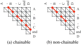
[image:4.612.103.265.60.152.2](a) chainable (b) non-chainable
Figure 5: A coordination with four conjuncts repre-sented as (a) chainable, and (b) non-chainable partial paths. We take (a) as the canonical representation.
3.2 Learning task
By the restriction of condition (iii) introduced above and the omission of (Outside, Substitute) from the node types, we can uniquely determine the com-plete path (from the initial node to the terminal node) that conjoins all the local alignments by Outside
nodes (which corresponds to edges in the original edit graph). In Figure 2, the augmented Outside
edges in this unique path are plotted as dotted lines for illustration.
Thus we obtain a complete path which is compat-ible with Collins’s perceptron-based sequence learn-ing method. The objective of the learning algo-rithms, which we will describe in Section 4, is to optimize the weight of features so that running the Viterbi algorithm will yield the same path as the gold standard.
Because a node in our state space corresponds to an edge in the original edit graph (see Figure 3), an arc in our state space is actually a pair of consec-utive edges (or equivalently, edit operations) in the original graph. Hence our model is more expressive than the original edit graph in that the score function can have a term (feature) defined on a pair of edit operations instead of one.
3.3 More complex coordinations
Even if a coordination comprises three or more con-juncts, our model can handle them, as it can be rep-resented as a set of pairwise local alignments that arechainable(Gusfield, 1997, Section 13.3). If pair-wise local alignments are chainable, a unique com-plete path that conjoins all these alignments can be determined, allowing the same treatment as the case with two conjuncts.
For instance, a coordination with four conjuncts
(A,B,CandD) can be decomposed into a set of pair-wise alignments{(A,B),(B,C),(C,D)}as depicted in Figure 5(a). This set of alignments are chain-able and thus constitute the canonical encoding for this coordination; any other pairwise decomposition for these four conjuncts, like{(A,B),(B,C),(A,D)}
(Figure 5(b)), is not chainable.
Our model can handle multiple non-nested coor-dinations in a single sentence as well, as they can also be decomposed into chainable pairwise align-ments. It cannot encode nested coordinations like (A,B, and (CandD)), however.
4 Algorithms
4.1 Reducing the cost of training data
construction
Our learning method is supervised, meaning that it requires training data annotated with correct labels. Since a label in our problem is local alignments (or paths in an edit graph) representing coordina-tions, the training sentences have to be annotated with word-by-word alignments.
There are two reasons relaxing this requirement is desirable. First, it is expensive to construct such data. Second, there are coordinate conjunctions in which word-by-word correspondence is unclear even for humans. In Figure 2, for example, a word-by-word alignment of ‘standard’ with ‘dense’ is de-picted, but it might be more natural to regard a word ‘standard’ as being aligned with two words ‘dose dense’ combined together.
Even if word-by-word alignment is uncertain, the boundaries of conjuncts are often obvious, and it is also much easier for human annotators to mark only the beginning and end of each conjunct. Thus we would like to allow for training examples in which only alignment boundaries are specified, instead of a full word-by-word alignment.
input: Set of examplesS={(xi,Yi)}
Iteration cutoffT
output: Averaged weight vector ¯w 1: ¯w←0;w←0
2: fort←1 . . .Tdo
3: Δw←0
4: for each(xi,Yi)∈Sdo
5: y←arg maxy∈Yiw·f(xi,y) 6: y←arg maxy∈A(xi)w·f(xi,y) 7: Δf←f(xi,y)−f(xi,y)
8: Δw←Δw+Δf 9: end for
10: ifΔw=0then
11: returnw¯ 12: end if
13: w←w+Δw 14: w¯←[(t−1)w¯+w]/t 15: end for
[image:5.612.75.221.59.255.2]16: returnw¯
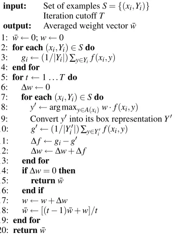
Figure 6: Path-based algorithm
this difficulty, we propose two simple heuristics we call the (i) path-based and (ii) box-based methods. As mentioned earlier, both of these methods are based on Collins’s averaged-perceptron algorithm for sequence labeling (Collins, 2002).
4.2 Path-based method
Our first method, which we call the “path-based” algorithm, is shown in Figure 6. We denote byA(x)
all possible alignments (paths) overx. The algorithm receivesT, the maximum number of iterations, and a set of examplesS={(xi,Yi)}as input, wherexiis a
sentence (a sequence of words with their attributes, e.g., part-of-speech, lemma, prefixes, and suffixes) andYi ⊂A(xi) is the set of admissible alignments
(paths) for xi. When a sentence is fully annotated with a word-by-word alignmenty,Yi={y}is a
sin-gleton set. In general boundary-only examples we described in Section 4.1,Yiholds all possible align-ments compatible with the marked range, or equiv-alently, paths that pass through the upper-left and lower-right corners of a rectangular region. Note that it is not necessary to explicitly enumerate all the member paths ofYi; the set notation here is only for
the sake of presentation.
The external function f(x,y) returns a vector (called theglobal feature vectorin (Sha and Pereira, 2003)) of the number of feature occurrences along the alignment pathy. In the beginning (line 5 in the figure) of the inner loop, the target path (alignment)
input: Set of examplesS={(xi,Yi)}
Iteration cutoffT
output: Averaged weight vector ¯w 1: ¯w←0;w←0
2: for each(xi,Yi)∈Sdo
3: gi←(1/|Yi|)∑y∈Yif(xi,y) 4: end for
5: fort←1 . . .Tdo
6: Δw←0
7: for each(xi,Yi)∈Sdo
8: y←arg maxy∈A(xi)w·f(xi,y) 9: Convertyinto its box representationY 10: g←(1/|Yi|)∑y∈Yif(xi,y)
11: Δf←gi−g
12: Δw←Δw+Δf 13: end for
14: ifΔw=0then
15: returnw¯ 16: end if
17: w←w+Δw 18: w¯←[(t−1)w¯+w]/t 19: end for
20: returnw¯
Figure 7: Box-based algorithm
is recomputed with the current weight vectorw. The arg max in lines 5 and 6 can be computed efficiently (O(n2), wherenis the number of words inx) by run-ning a pass of the Viterbi algorithm in the edit graph forx. The weight vectorwvaries between iterations, and so does the most likely alignment with respect tow. Hence the recomputation in line 5 is needed.
4.3 Box-based method
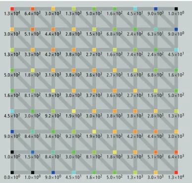
Our next method, called “box-based,” is designed on the following heuristic. Given a rectangle region representing a local alignment (hence all nodes in the region are of polarity Inside) in an edit graph, we distribute feature weights in proportion to the probability of a node (or an arc) being passed by a path from the initial (upper left) node to the termi-nal (lower right) node of the rectangle. We assume paths are uniformly distributed.
[image:5.612.316.492.60.297.2]Figure 8: Number of paths passing through the ver-tices of an 8×8 grid.
towards alignments with a larger number of substi-tutions.
The pseudo-code for the box-based algorithm is shown in Figure 7. For each examplexiand its
pos-sible target labels (alignments)Yi, this algorithm first (line 3) computes and stores in the vectorgithe
aver-age number of feature occurrences in all possible tar-get paths inYi. This quantity can be computed sim-ply by summing over all nodes and edges feature oc-currences multiplied by the pre-computed frequency of each nodes and arcs at which these features occur. analogously to the forward-backward algorithm. In each iteration, the algorithm scans every example (lines 7–13), computing the Viterbi path y (line 8) according to the current weight vector w. Line 9 then convertsy to its box representationY, by se-quentially collapsing consecutiveInsidenodes iny
as a box. For instance, lety be the local alignment depicted as the bold line in Figure 2. The boxY
computed in line 9 for thisyis the shaded area in the figure. In parallel to the initialization step in line 3, we store ing the average feature occurrences inY
and update the current weight vectorwby the differ-ence between the targetgi andg. These steps can be interpreted as a Viterbi approximation for com-puting the optimal setYof alignments directly.
5 Related work
5.1 Discriminative learning of edit distance
In our model, the state space of sequence alignment, or edit graph, is two-dimensional (which is actu-ally three-dimensional if the dimension for labels is taken into account). This is contrastive to the one dimensional models used by Collins’s perceptron-based sequence method (Collins, 2002) which our algorithms are based upon, and by the linear-chain CRFs.
McCallum et al. (McCallum et al., 2005) pro-posed a CRF tailored to learning string edit distance for the identity uncertainty problem. The state space in their work is two dimensional just like our model, but it is composed of two decoupled subspaces, each corresponding to ‘match’ and ‘mismatch,’ thus shar-ing only the initial state. It is not possible to make a transition from a state in the ‘match’ state space to the ‘mismatch’ space (and vice versa). As we can see from the decoupled state space, this method is based on global alignment rather than local align-ment; it is not clear whether their method can iden-tify local homologies in sequences. Our method uses a single state space in which both ‘match (inside)’ and ‘mismatch (outside)’ nodes co-exist and transi-tion between them is permitted.
5.2 Inverse sequence alignment in
computational biology
In computational biology, the estimation of a sub-stitution matrix from data is called the inverse se-quence alignment problem. Until recently, there have been a relatively small number of papers in this field despite a large body of literature in se-quence alignment. Theoretical studies in the inverse sequence alignment include (Pachter and Sturmfels, 2004; Sun et al., 2004). Recently, CRFs have been applied for optimizing the substitution matrix in the context of global protein sequence alignment (Do et al., 2006).
6 Empirical evaluation
6.1 Dataset and Task
We used the GENIA Treebank beta corpus (Kim et al., 2003)2 for evaluation of our methods. The
pus consists of 500 parsed abstracts in Medline with a total of 4529 sentences.
Although the Penn Treebank Wall Street Journal (WSJ) is the de facto standard corpus for evaluating chunking and parsing performance, it lacks adequate structural information on coordinate conjunctions, and therefore does not serve our purpose. Many coordinations in the Penn Treebank are given a flat bracketing like (A, B, and C D), and thus we cannot tell which of ((A, B, and C) D) and ((A), (B), and (C D)) gives a correct alignment. The GENIA cor-pus, in contrast, distinguishes ((A, B, and C) D) and ((A), (B), and (C D)) explicitly, by providing more detailed bracketing. In addition, the corpus contains an explicit tag “COOD” for marking coordinations.
To avoid nested coordinations, which admittedly require techniques other than the one proposed in this paper, we selected from the GENIA corpus sen-tences in which the conjunction “and” occurs just once. After this operation, the number of sentences reduced to 1668, from which we further removed 32 that are not associated with the ‘COOD’ tag, and 3 more whose annotated tree structures contained obvious errors. Of the remaining 1633 sentences, 1061 were coordinated noun phrases annotated with NP-COOD tags, 226 coordinated verb phrases (VP-COOD), 142 coordinated adjective phrases (ADJP-COOD), and so on. Because the number of VP-COOD, ADJP-VP-COOD, and other types of coordi-nated phrases are too small to make a meaningful benchmark, we focus on coordinated noun phrases in this experiment.
The task hence amounts to identifying coordi-nated NPs and their constituent conjuncts in the 1633 sentences, all of which contain a coordination marker “and” but only 1061 of which are actually coordinated NPs.
6.2 Baselines
We used several publicly available full parsers as baselines: (i) the Bikel parser (Bikel, 2005) version 0.9.9c with configuration file
bikel.properties (denoted as Bikel/Bikel),
(ii) the Bikel parser in the Collins parser emula-tion mode (using collins.properties file) (Bikel/Collins), and (iii) Charniak and Johnson’s reranking parser (Charniak-Johnson) (Charniak and Johnson, 2005). We trained Bikel’s parser and its
Collins emulator with the GENIA corpus, WSJ, and the combination of the two. Charniak and Johnson’s parser was used as distributed at Charniak’s home page (and is WSJ trained).
Another baseline we used is chunkers based on linear-chain CRFs and the standard BIO la-bels. We trained two types of CRF-based chun-kers by using different BIO sequences, one for the conjunct bracketing and the other for coor-dination bracketing. The chunkers were imple-mented with T. Kudo’s CRF++ package version 0.45. We varied its regularization parameters C
amongC∈ {0.01,0.1,1,10,100,1000}, and the best results among these are reported below.
6.3 Features
Letx= (x1,...,xn) be a sentence, with its member
xk a vector of attributes for the kth word. The
at-tributes include word surface, part-of-speech (POS), and suffixes, among others.
Table 1 summarizes (i) the features assigned to a node whose corresponding edge in the original edit graph forxis emanating from row iand column j, and (ii) the features assigned to the arcs (consisting of two edges in the original edit graph) whose joint (the vertex between the two edges) is a vertex at row
iand column j.
We also tested the path-based and box-based methods, and the CRF chunkers both with and with-out the word and suffix features.
Although this is not a requirement of our model or algorithms, every feature we use in this experiment is binary; if the condition associated with a feature is satisfied, the feature takes a value of 1; otherwise, it is 0. A condition typically asks whether or not specific attributes match those at a current node, arc, or their neighbors.
We used the POS tags from the GENIA corpus as the POS attribute. The morphological features include 3- and 4-gram suffixes and indicators of whether a word includes capital letters, hyphens, and digits.
Table 1: Features for the proposed methods
Substitute(diagonal) nodes (∗,Substitute,∗)
Indicators of the word, POS, and morphological attributes ofxi,xj,(xi−1,xi),
(xi,xi+1), (xj−1,xj),(xj,xj+1), and(xi, xj), respectively combined with the
type of the node.
For each of the word, POS, and morphological attributes, an indicator of whether the respective attribute is identical inxi andxj, combined with the
type of the node.
Delete(vertical) nodes (∗,Delete,∗)
Indicators of the word, POS, and morphological attributes of xi, xj, xj−1,
(xi−1,xi),(xi,xi+1), and(xj−1,xj), combined with the type of the node. Insert(horizontal) nodes
(∗,Insert,∗)
Indicators of the word, POS, and morphological attributes of xi, xi−1, xj,
(xi−1,xi),(xj−1,xj), and(xj,xj+1), combined with the type of the node.
Any arcs
(∗,∗,∗)→(∗,∗,∗) Indicators of the POS attribute of(xi,xi+1),(xj−2,xj−1),(xj−1,xj),(xxji,,xxji+−11),,(xxji,−x1,j−x1j−,1()x,i−(x2i,−x1i−,x1j)),,((xxii−,x1,j−xi1)), and(xi,xj), combined with the type pair of the arc.
Arcs between nodes of different polarity (∗,Inside,∗)→(∗,Outside,∗)and
(∗,Outside,∗)→(∗,Inside,∗)
Indicator of the distancej−ibetween two wordsxiandxj, combined with the
type pair of the arc.
and jin Table 1. The latter cannot be incorporated as a local features in chunkers based on linear chain.
For the Bikel (and its Collins emulation) parsers which accepts POS tags output by external taggers upon testing, we gave them the POS tags from the GENIA corpus, for fair comparison with the pro-posed methods and CRF-based chunkers.
6.4 Evaluation criteria
We employed two evaluation criteria: (i) correctness of the conjuncts output by the algorithm, and (ii) cor-rectness of the range of coordinations as a whole.
For the correctness of conjuncts, we further use two evaluation criteria. The first evaluation method (“pairwise evaluation”) is based on the decomposi-tion of coordinadecomposi-tions into the canonical set of pair-wise alignments, as described in Section 3.3. After the set of pairwise alignments is obtained, each pair-wise alignment is transformed into a box surrounded by their boundaries. Using these boxes, we evaluate precision, recall and F rates through the following definition. The precision measures how many of the boxes output by the algorithm exactly match those in the gold standard, and the recall rate is the per-centage of boxes found by the algorithm. The F rate is the harmonic mean of the precision and the recall.
The second evaluation method (“chunk-based evaluation”) for conjuncts is based on whether the algorithm correctly outputs the beginning and end of each conjunct, in the same manner as the chunking tasks. Here, we adopt the evaluation criteria for the
CoNLL 99 NP bracketing task3; the precision equals how many of the NP conjuncts output by the algo-rithm are correct, and the recall is the percentage of NP conjuncts found by the algorithm.
Of these two evaluation methods for conjuncts, it is harder to obtain a higher pairwise evaluation score than the chunk-based evaluation. To be counted as a true positive in the pairwise evaluation, two consec-utive chunks must be output correctly by the algo-rithm.
For the correctness of the coordination range, we check if both the start of the first coordinated con-junct and the end of the last concon-junct in the gold match those output by the algorithm The reason we evaluate coordination range is to compare our pro-posed method with the full parsers trained on WSJ (but applied to GENIA). Although WSJ and GE-NIA differ in the way conjuncts are annotated, they are mostly identical on how the range of coordina-tions are annotated, and hence comparison is feasi-ble in terms of coordination range. For the baseline parsers, we regard the bracketing directly surround-ing the coordination marker “and” as their output.
In (Clegg and Shepherd, 2007), an F score of 75.5 is reported for the Bikel parser on coordination de-tection. Their evaluation is based on dependencies, which is different from our evaluation criteria which are all based on boundaries. Generally speaking, our evaluation criterion seems stricter, as exemplified in Figures 7 and 8 of Clegg and Shepherd’s paper; in these figures, our evaluation criterion would result
Table 2: Performance on conjunct bracketing. P: precision (%), R: recall (%), F: F rate.
Pairwise evaluation Chunk-based evaluation
Method P R F P R F
Path-based method 61.4 56.2 58.7 70.9 66.9 68.9 Path-based method without word and suffix features 61.7 58.8 60.2 71.2 69.7 70.5
Box-based method 60.6 58.3 59.4 70.5 69.1 69.8 Box-based method without word and suffix features 59.5 58.3 58.9 69.7 69.5 69.6 Linear-chain CRF chunker (conjunct bracketing) 62.6 51.4 56.4 71.0 66.1 68.5 Bikel/Collins, trained with GENIA 50.0 48.6 49.3 65.0 64.2 64.6 Bikel/Bikel, trained with GENIA 50.1 47.8 49.0 63.9 61.3 62.6
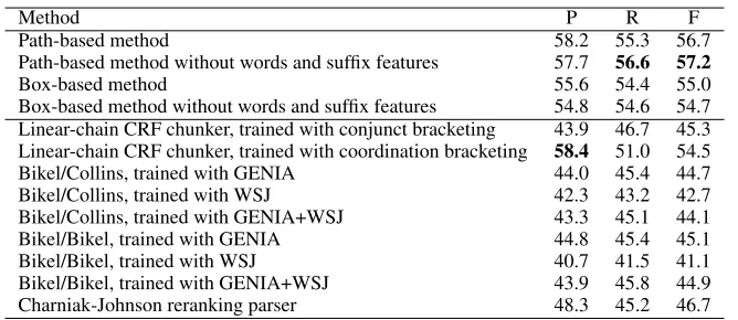
Table 3: Performance on coordination bracketing. P: precision (%), R: recall (%), F: F rate.
Method P R F
Path-based method 58.2 55.3 56.7
Path-based method without words and suffix features 57.7 56.6 57.2
Box-based method 55.6 54.4 55.0
Box-based method without words and suffix features 54.8 54.6 54.7 Linear-chain CRF chunker, trained with conjunct bracketing 43.9 46.7 45.3 Linear-chain CRF chunker, trained with coordination bracketing 58.4 51.0 54.5 Bikel/Collins, trained with GENIA 44.0 45.4 44.7 Bikel/Collins, trained with WSJ 42.3 43.2 42.7 Bikel/Collins, trained with GENIA+WSJ 43.3 45.1 44.1 Bikel/Bikel, trained with GENIA 44.8 45.4 45.1 Bikel/Bikel, trained with WSJ 40.7 41.5 41.1 Bikel/Bikel, trained with GENIA+WSJ 43.9 45.8 44.9 Charniak-Johnson reranking parser 48.3 45.2 46.7
in zero true positive, whereas their evaluation counts the dependency arc from ‘genes’ to ‘human’ as one true positive.
6.5 Results
The results of conjunct and coordination bracketing are shown in Tables 2 and 3, respectively. These are the results of a five-fold cross validation. We ran the proposed methods until convergence or the cutoff iteration ofT=10000, whichever comes first. The path-based method (without words and suf-fixes) and box-based method (with full features) each achieved 2.0 and 1.3 point improvements over the CRF chunker in terms of the F score in conjunct identification (chunk-based evaluation), 3.8 and 3.0 point improvement in terms of pairwise evaluation, and 2.7 and 0.5 points in coordinate identification, respectively. Our methods also showed a perfor-mance considerably higher than the baseline parsers. The performance of the path-based method was better when the word and suffix features were re-moved, while the box-based method and CRF chun-kers performed better with these features.
7 Conclusions
We have proposed a new coordination learning and disambiguation method that can incorporate many different features, and automatically optimize their weights on training data.
In the experiment of Section 6, the proposed method obtained a performance superior to a linear-chain chunker and to the state-of-art full parsers.
[image:9.612.141.475.217.362.2]References
Rajeev Agarwal and Lois Boggess. 1992. A simple but useful approach to conjunct identification. In Proceed-ings of the 30th Annual Meeting of the Association for Computing Linguistics (ACL’92), pages 15–21.
Daniel M. Bikel. 2005. Multilingual statistical pars-ing engine version 0.9.9c. http://www.cis.upenn.edu/
∼dbikel/software.html.
Francis Chantree, Adam Kilgarriff, Anne de Roeck, and Alistair Willis. 2005. Disambiguating coordina-tions using word distribution information. In Pro-ceedings of the International Conference on Recent Advances in Natural Language Processing (RANLP 2005), Borovets, Bulgaria.
Eugene Charniak and Mark Johnson. 2005. Coarse-to-finen-best parsing and MaxEnt discriminative rerank-ing. InProceedings of the Annual Meeting of the As-sociation for Computational Linguistics (ACL-2005).
Andrew B Clegg and Adrian J Shepherd. 2007. Bench-marking natural-language parsers for biological appli-cations using dependency graphs. BMC Bioinformat-ics, 8(24).
Michael Collins. 2002. Discriminative training meth-ods for hidden Markov models: theory and experi-ments with perceptron algorithms. InProceedings of the Conference on Empirical Methods in Natural Lan-guage Processing (EMNLP 2002).
C. B. Do, S. S. Gross, and S. Batzoglou. 2006. CON-TRAlign: discriminative training for protein sequence alignment. InProceedings of the Tenth Annual Inter-national Conference on Computational Molecular Bi-ology (RECOMB 2006).
Dan Gusfield. 1997. Algorithms on Strings, Trees, and Sequences. Cambridge University Press.
J.-D. Kim, T. Ohta, Y. Tateisi, and J. Tsujii. 2003. GE-NIA corpus: a semantically annotated corpus for bio-textmining. Bioinformatics, 19(Suppl. 1):i180–i182.
Sadao Kurohashi and Makoto Nagao. 1994. A syntactic analysis method of long Japanese sentences based on the detection of conjunctive structures. Computational Linguistics, 20:507–534.
John Lafferty, Andrew McCallum, and Fernando Pereira. 2001. Conditional random fields: probabilistic mod-els for segmenting and labeling sequence data. In Pro-ceedings of the 18th International Conference on Ma-chine Learning (ICML-2001), pages 282–289. Morgan Kaufmann.
Andrew McCallum, Kedar Bellare, and Fernando Pereira. 2005. A conditional random field for discriminatively-trained finite-state string edit distance. InProceedings
of the 21st Conference on Uncertainty in Artificial In-telligence (UAI-2005).
Preslav Nakov and Marti Hearst. 2005. Using the web as an implicit training set: application to structural ambi-guity resolution. InProceedings of Human Language Technology Conference and Conference on Empirical Methods in Natural Language (HLT/EMNLP), pages 835–842, Vancouver.
Akitoshi Okumura and Kazunori Muraki. 1994. Sym-metric pattern matching analysis for English coordi-nate structures. InProceedings of the Fourth Confer-ence on Applied Natural Language Processing, pages 41–46.
Lior Pachter and Bernd Sturmfels. 2004. Parametric inference for biological sequence analysis. Proceed-ings of the National Academy of Sciences of the USA, 101(46):16138–16143.
Philip Resnik. 1999. Semantic similarity in a taxonomy: an information-based measure and its application to problems of ambiguity in natural language. Journal of Artificial Intelligence Research, 11:95–130.
Fei Sha and Fernando Pereira. 2003. Shallow pars-ing with conditional random fields. In Proceedings of the Human Language Technology Conference North American Chapter of Association for Computational Linguistics (HLT-NAACL 2003), pages 213–220, Ed-monton, Alberta, Canada. Association for Computa-tional Linguistics.