Quantile Regression Based on Semi-Competing
Risks Data
Jin-Jian Hsieh1, A. Adam Ding2, Weijing Wang3, Yu-Lin Chi1 1Department of Mathematics, National Chung Cheng University, Chia-Yi, Chinese Taipei
2Department of Mathematics, Northeastern University, Boston, USA 3Institute of Statistics, National Chiao-Tung University, Hsin-Chu, Chinese Taipei
Email: [email protected], [email protected], [email protected] Received December 7,2012; revised January 10, 2013; accepted January 22,2013
ABSTRACT
This paper considers quantile regression analysis based on semi-competing risks data in which a non-terminal event may be dependently censored by a terminal event. The major interest is the covariate effects on the quantile of the non-terminal event time. Dependent censoring is handled by assuming that the joint distribution of the two event times follows a parametric copula model with unspecified marginal distributions. The technique of inverse probability weighting (IPW) is adopted to adjust for the selection bias. Large-sample properties of the proposed estimator are de- rived and a model diagnostic procedure is developed to check the adequacy of the model assumption. Simulation results show that the proposed estimator performs well. For illustrative purposes, our method is applied to analyze the bone marrow transplant data in [1].
Keywords: Copula Model; Dependent Censoring; Quantile Regression; Semi-Competing Risks Data
1. Introduction
Quantile regression analysis has received increasing at- tentions in the recent literature of survival analysis. Compared with conventional regression models such as the proportional hazards (PH) model or the accelerated failure time (AFT) model, quantile regression models provide direct assessment of the covariate effect on dif- ferent quantiles of the failure time variable. This model also allows covariates to affect both location and shape of the distribution. Let T be the failure time of interest, be a vector and . Consider the following linear quantile regression model on Z
p1 Z
1, T
TZ
h T
, where h
is a known monotonic function, such that
β0
Z,T h T
Z
0 1
(1) where and
Y Z
is the
100
th quantile of Y conditional on Z. Note that when we set, model (1) is equivalent to
T
0
h T β Z
Pr 0 Z . Many papers for estimating β0
without specifying the distribution of T Z or have appeared in the literature. [2-5] considered quantile re- gression analysis under a fixed censoring mechanism in which all the censoring times are observed. Independent right censorship has been assumed by many papers in- cluding [6-11].
In this paper, we consider semi-competing risks data
[12] in which the failure time of a non-terminal event T is subject to dependent censoring by a terminal event time
D but not vice versa. Consider an example of bone mar- row transplantation for leukemia patients described in [1] such that T is the time to leukemia relapse and D is the time to death. One important risk factor is the disease classification (i.e. ALL, AML low-risk, and AML high- risk) which was determined based on patient’s status at the time of transplantation. Here we assume that T, the time to a non-terminal event, follows model (1). Note that [13,14] also considered quantile regression analysis for competing risks data and left-truncated semi-com- peting risks data respectively. They defined the quantiles based on the crude quantity, namely the cumulative inci- dence function Pr
T t T , D
. In contrast, the pro- posed regression model (1) is defined based on the netquantity Pr
T t
which is not identifiable withoutextra assumption on the dependence structure. There has been some controversy over which quantity should be used in presence of dependent competing risks. We be- lieve that both quantities are important and not mutually exclusive as they provide information on different as- pects of the data. Here β0
measures the covariate effect on T after separating the potential influence fromD. Such analysis is also useful in practical applications. For example, a covariate may prolong D so that increase
Pr T t T , D but have no direct effect on the non-
terminal event. The dependence between T and D com- plicates the estimation of β0
X Y, , X, Y
. We will adopt a semi-parametric copula assumption to model their joint distribution and apply the technique of inverse probabil- ity weighting (IPW) to correct the bias due to dependent censoring in the estimation procedure. The association parameter in the copula model will also be estimated using existing methods.
The rest of this paper is organized as follows. In Sec- tion 2, we introduce the data structure and model as- sumptions. The proposed methodology for parameter estimation and model checking is presented in Section 3. The proofs of the asymptotic properties are given in the Appendix. Section 4 contains simulation results. In Sec- tion 5, we apply the proposed methods to analyze the bone marrow transplant data in [1] and in Section 6, we give some concluding remarks.
2. Data and Model Assumptions
Recall that T and D denote the time to a non-terminal event and the time to a terminal event respectively such that T is subject to censoring by D but not vice versa. In presence of additional external censoring due to drop-out or the end-of-study effect, one observes such that X T D C, Y D C, XI T
D C
,
Y I D
C , where is the minimum operator and I is the indicator function. The covariate vectors can be denoted as Z
p1 and . The sample
Z
1,Z
T T
Contains
X Yi, ,i Xi, Yi,Zi i1, ,n
X Y, , , ,Z
0
which are ran- dom replications of X Y . We will assume that and C are independent given Z. The covari-ate effect on T is specified by model (1) and the major objective is to estimate
T D,
β based on semi-compet- ing risks data.
To handle dependent censoring, we have to make extra assumptions about the dependence structure between T
and D in the upper wedge. According to [15] who ex- tended Sklar’s theorem to the regression setting, we con- sider the following copula model
Tz
t S, Dz
d
,
Pr T t D d, Z z Cz S (2)
where 0 t d ,STz
t and SDz
d are the mar- ginal survival functions of T and D, given Zz, andis a parametric copula function defined on the unit square. The association parameter
, C
in (2) is related to Kendall’s tau defined by
1 1
0 0
4 C u v,
C
d ,du v
1.
In particular, we will assume T D Z, in the upper wedge follows a popular subclass of copula models, namely Archimedean copula (AC), in which the copula
function can be further expressed as
, 1
, 0 , 1,C u v u v u v (3)
where is a non-increasing convex function defined on
0,1
with
1 0. Examples of Archimedean copula include Clayton’s copula with
s s 1
and
1
, 1
C u v uv ;
and Frank’s copula with
s log 1
log 1
s
and
, log 1 u 1 v 1 1
C u v .
3. The Proposed Inference Methods
Our major objective is to develop an inference method for estimation 0
but, in the mean time, employ existing methods for estimating based on semi- competing risks data such as those proposed by [16] and [17].
β
3.1. Estimation of
for Discrete Covariates
0
In absence of censoring, one can estimate β by solving
1 2 T
1
0.
n
i i i
i
n I h T
Z β Zi
T DiC
Since is subject to censoring by i, it follows
that
T 0
T 0
T 0
,
,
i
i
i
i
i i X
i i
i i X
i i i
i
i i i
I h X E
H X
I h T
E E T
H T E I h T
Z
Z
β Z
Z
β Z
Z Z
β Z Z
where the reciprocal of the weight function is given by
,
Pr 1 ,
Pr ,
Pr Pr ,
.
X
D T
H t T t
D C t T t
C t D t T t
G t S t
Z
Z Z
Z Z
Z Z
OJS
0
Copyright © 2013 SciRes.
function for β Kaplan-Meier estimator based on data
T 1 2 1 i n i i i i iI h X n H X
z β ZZ Xi 0.
This is the so called inverse probability weighting tech- nique for bias correction. Since Hzi Xi needs to be estimated, it is natural to modify the estimating equa- tion as
T 1 2 1 , ˆ i nn i i
i
i i
S
I h X n H X
z β β ZZ Xi 0,
(4)
where the estimated components in the weight can be denoted as
, ˆ ˆ ˆ Pr > Pri i i
z i i D T
i i i
i i
H X G X S
C X
D X T
z z Z
, . i ii i i i
X
z
X z
Z
C
Now we discuss estimation of the weight components. We will first address the situation that Z takes discrete values, and then briefly discuss possible modification for continuous covariates. Since is independent of T and
D given Z, Pr
CxZz
can be estimated by the
Yi,1Yi
i1, , n
or
Xi,1 Xi Yi
i1, , n
zwith Zi . We will utilize some analytic properties of the chosen AC model to derive an explicit expression of
Pr D x T x,Zi . Denote ST z,
x Pr
TxZ z
,
, Pr
D
S z x D x Z z and
, Pr
W
S z x W T D xZz . It follows that
, , , , , 1 , 1 , , , Pr , .u ST D
u ST D
D T
x v S x
x v S x T
W
S x D x T x
u v u u u v S x S x z z z z z
z z z
z
z z z z
z z
z z
Z z
We suggest to estimate S
x
, ˆ
W
S z x
,
D Tz by applying the es- timators in [17] for quantities in the right-hand side of the above expression. Specifically is the Kap- lan-Meier estimator of Pr
T D x Zz
based on
Xi,Wi
i1, , n
, where Wi I T
iDi<Ci
,
, ˆ
T
S z x
ˆ ,
ˆ ,
ˆ , 1, ˆ ˆ ,
i
n
X i W i W i
x S X S X
is the copula-graphic estimator
1, ˆ
1
T z i
i
S x I X
z z
z Z z z z
ˆ
z
where the estimator is the root of the following estimating equation,
, i j
i j Z Z
ˆ
π ,
, > 0 0,
ˆ
π , 1
ij ij
ij i j i j
ij ij
X Y
C I X X Y Y
X Y z z
z z z
ij ij ij ij
w X Y I T D
where XijXiXj Yij Y Yi j ij i j
D D D
ij i j
C C C w
,
, , ij i j, , , is a weight func-
T T T tion, z v vz v z v , and
1
ˆ
π , Pr ,
ˆ
> , > , ,
n
i i i z z
i
s t T s D t
I X x Y y Z z n G y
z Z z
1
n
z i
j
n I Z z
where . Then
, ˆ , , ˆ ˆ ˆ . ˆ T D T W S x S x S x z z z z z (5)
This estimator is then used in estimating Equation (4). The Equation (4) may not be continuous so that an exact solution may not exist. Here we define βˆ
as a generalized solution as in [13,18]. By the monotonic property of (4), the set of generalized solutions is convex. Using the arguments in [13], the solution of (4) can be reformulated as the minimizer of the following function,
T T T
1 1 1
, ˆ ˆ ˆ l 2 ,
i
i i
n n n
l X
i i
n X k
i z i z i l z l k
l
h X
U M M
H X H X H X
Z
Z
b b b b Z
where M is a large enough positive value to bound
T n l Xl 1 ˆ l
i Hz Xl
Zb and T n
2
1 k
k
We suggest using a re-sampling approach for variance es
b Z from above.
timation since the analytic formula for the variance of
ˆ
β is complicated to calculate. Based on the non- parametric bootstrap approach, we can sample replica- tions
X Yi , ,i xi, yi
i1, ,n
from the original data. Given a bootstrap sample, we can compute βˆ
. Re- peating the re-sampling procedure B times, btain
ˆ : 1, ,
b b B
β and the variance of ˆ
we o
β can be estimated by
2
,
B
β βˆ
1
1 ˆ
1
B b b
V
where
=ˆ
B b i b
B
β β . Furthermore, we can con- the
1
struct confidence interval for β
as
1 2 ˆˆ V z
12
β , where z12 1
1 2
, and
is the cumulative distribution function of a standard normal random variable. The bootstrap percentile method suggests another way of constructing a
1
confi- dence interval of β
with the formula 2
1 2
ˆ ,ˆ
B B
β β , where βˆ b
, b1, , Bare the order statistics of βˆb
for b1, , B.es for Discrete
We consistency and weak conver- 3.2. Asymptotic Properti
Covariates establish the uniform
gence of the proposed estimator βˆ
for
L, U
,a region that 0
is identifia e first st regularity condi(C1) Denote the set of possible covariate Z values as
ble. W ate the tions.
which is a compact set in p1. The probability nsity function fZ
z for cov e Z is uniformlybounded above and belo on .
(C2) There exists a compact set in the parameter sp
de ariat
w
ace for the copula parameter such that all true values of
z are interior points o f for all z.(C3) There exists 0 such that Pr
C
,P
0 0
r C 0, infzST,
SD,
z . z
and
1sup ST,z SD,z
z
(C4) 1) β0 is Lipschitz continuous for
L, U
;2) The density T,
d T,
df z t S z t is bou e
t nded abov
uniformly for t
0, and z; 3) The copula gen- erator function
u has continuous derivatives
u ,
u
,
u ,
u
u and
u which do not e r all
qual 0 fo and u
0,1
.(C5)
0
infb eigmin A b
c0, for some 00 and c 0, wh e
2 1 T,
T
E h
Z
A b Z Z
0 er
b
,
1
, L U
0
: inf
p
B bR bβ ,
2 T
u a vector u.
Condition C1 assumes the boundedness of covariates and is satisfied for finite discrete covariates. T as- sumption is only used to derive the asymptotic prop and uu for
his erties of ˆDT,z for p Condition C2 assumes th
S roving Theorem 1.
at the true value of is an interior point in the pa- rameter space which is a common regularity condition. Condition C3 is assumed to simplify theoretical argu-ments similar to condition C1 in [13], and generally
is the study end time in ractical applications. Conditions C4 1) and 2) assume the smoothness of coefficient proc- esses, and the uniform boundedness on the density of T, which are standard for quantile regression methods. Condition C4 3) imposes the smoothness requirement on the copula generator function similar to the regularity conditions in [17,19]. Condition C5 is similar to condi-tion C4 in [13] which ensures the identifiability of
p
0
β and is needed for proving the consistency of
ˆ β .
Therefore with finite , we prove the following result.
Theorem 1 If conditions C1-C5 hold, then
,
0
m sup 0
L U
n ,
and
ˆ p
β β
li
ˆ
1 2
n 0 mean-
ze
The detailed proofs are presented in the Appen x. Model Checking
[20-22] in which complete data ar
β β converges weakly to a ro Gaussian process.
di 3.3. and Model Diagnosis Motivated by the work of
e considered, we define the residual quantities as
ˆT
i i
i i i X z i
e I h X H X
β Z
for i1, , n and consider
1
,
n i i
i
n1 2 n q e
Z
re q
whe i ed weight function. Simi-
o the argu n
s a known bound
lar t ments in [13,23], converges weakly to a zero-mean Gaussian process if model (1) is specified correctly and the covariate takes discrete lues. There- va fore we propose the following test statistic
1 2
1
, ˆ
n n
i e
q e
T n i i
Z
n
which can be obtained by applying the bootstrap approach mentioned earlier. Thus, we have that Tn con-
verges to the standard normal random variable asymp- totically as the model is correct. On the o er hand, when the model is mis-specified, Tn will deviate from zero.
ing
th
Accord ly we can reject the model assumption if 2
n Z , where
T Z2 is the quantile of N
0,1 and is the level of significance. If there are K candidate models under consideration, we compute the absolute value of Tn for each model for k1, , K and choose
the one with the smallest value.
mation for Continuous Covaria
We briefly discuss how to extend our estimation method for continuous covariates. One can apply a smoothing approach to estimate the proba tions condi- tional on z. Following [24], wi
3.4. Esti tes
ility func
ss of generality, b
thout lo
assume that Z
0,1 and Z1Z2Zn adered. Let
re or-
1
0
1 1
d , 1, , , ,
1
, d ,
i n
n n t Z n n Z
n n
n n t Z
z t
K t i n
c z h h h
z t
c z h K t
h h
where Z0 0 ,
i
Z ni n
w z h
, hn0 is the bandwidth and K is the kernel. Then
W i
, 1
1
,
ˆ 1 ,
1 ,
i
n n i
W z i
W x
n n i j
w z h S x
w z h
where
W i ,W i ,wn i
z h, n
i1, , n
are the re-ment
arrange
sorted ac-cording t
, i, , 1, ,
i W ni n
W w z h i n o Wi, where WiTiDi and
i
W I Ti Di i
ula-graphic
estimator in [24] C
, and SˆT,z
x is the cop
, ˆ ,
ˆ ˆ , ,
W i W i ni n
S X w z h
1
, ˆ ˆ
1
ˆ , 1
i
n
T z i X
i
S x I X x
X S
z z z (6)
z z
and ˆ
z solves estimating equation
ˆ
π ,
, 0
ˆ
π , 1
z ij ij j
i
ij ij ij ij i j i j
z ij ij
X Y z Z
z Z
K K Y I T D C I X X Y Y
X Y
z
z
he asymptotic covariates. For ex-
ons of
0.
ij
w X
d to derive t ntinuous
thed versi
i j hn hn
Special techniques are neede properties for the case of co ample properties of the smoo
0 1
log T b b 1Z , (8) where Z Ber 0.5
,
b b0, 1
1.5, 0.5
and ,ˆ
D T
S z and
z ˆ are not fully available yet. The n1 2 convergence rate for the normality proof may not be directly extended since the smooth version of SˆD T,z may not be n1 2 asymptotic normal. However the estimator for uan-
gression parameter may still be
the q
tile re n1
erformance of the proposed methods with R 2 asymptotic normal even when some component converges at a slow- er rate.
4. Simulation Studies
We conduct simulation studies to examine the finite- sample p
software. Here we consider we consider the model,
two cases. For the first one,
1
2
0 0
log T Z, (7) where ZBer 0.5
and 0
0
ich follow the Clayton copula
and Frank copula with
1 , 2
1, 1
.We generate
,D
wh
marginally follow
0.5 , 0.5 0.5
U
ing
so that Pr
0
, and ginally following exp(2) t nd case, we con- siderD mar- . For he seco
,D
generated from the Clayton copula and Frank copula following
with U
and Dexp 2
. In this
0, 0.5case,
1
0 0 b0 0.5b1 , 0.5b12
,
. Three lev- els of association τ = 0.3, 0.5, 0.7 are considered
follows istribution on
. The censoring variable C a uniform d
0,12
.We evaluate the performances for γ= 0.1, 0.3, 0.5 and d on 400 sim
the proposed r, we the sample size n = 100 base
he standard e r of ulation runs. To
obtain t rro estimato
use the bootstrap method with B = 50. Based on the set- tings, we also present a naive estimator of β0
, which is con tructed under ths e wrong assumption that T is in-at is,
dependently censored by D C . Th we estimate
0
β by solving the estimating Equation (4) with
1
1
,
.
n
j j i j i j
n
j i j
ˆ Pr
Hzi Xi D C X Zi zi
I D C X Z z
I Z z
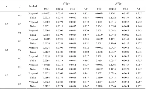
Tables 1-4 report the average bias of the proposed
[image:6.595.60.538.102.394.2]
sults f ression parameters under model (7) with Clayton copula.
Table 1. Finite-sample re or estimating the quantile reg 1
ˆ ˆ 2
τ γ Method
Bias EmpSd MSE CP Bias EmpSd MSE CP
Proposed 0.0059 0.0263 0.0007 0.975 0.0011 0.0369 0.0013 0.980
0.1
Naive 0.0129 0.0284 0.0009 0.975 −0.0019 0.0380 0.0014 0.975
Proposed 0.0024 0.0383 0.0014 0.940 −0.0001 0.0498 0.0024 0.945
0.3
Naive 0.0183 0.0379 0.0017 0.947 −0.0115 0.0487 0.0025 0.942
14 0.935 0.0024 0.0546 0.0029 0.922 0.3
Proposed 0.0074 0.0300 0009 0.955 −0.0007 0.0422 0.962
Proposed 0.0001 0.0380 0.00
0.5
Naive 0.0163 0.0386 0.0017 0.915 −0.0078 0.0554 0.0031 0.930
0. 0.0017
0.1
0 0. 0. −0. 0. 0.
−
−
0.5
−
Naive .0240 0.0318 0015 891 0124 0.0404 0017 932
Proposed 0.0064 0.0391 0.0015 0.925 0.0024 0.0500 0.0025 0.962
0.3
Naive 0.0369 0.0384 0.0028 0.817 −0.0232 0.0511 0.0031 0.922
Proposed 0.0001 0.0381 0.0014 0.912 0.0025 0.0497 0.0024 0.957
0.5
Naive 0.0259 0.0357 0.0019 0.867 −0.0139 0.0495 0.0026 0.942
Proposed 0.0087 0.0323 0.0011 0.945 0.0008 0.0440 0.0019 0.967
0.1
Naive 0.0420 0.0335 0.0028 0.802 −0.0260 0.0432 0.0025 0.920
Proposed 0.0073 0.0371 0.0014 0.925 0.0004 0.0519 0.0026 0.927
0.3
Naive 0.0475 0.0358 0.0035 0.707 −0.0254 0.0528 0.0034 0.902
Proposed 0.0065 0.0378 0.0014 0.937 −0.0029 0.0521 0.0027 0.945
0.7
0.5
Naive 0.0314 0.0344 0.0021 0.845 −0.0159 0.0477 0.0025 0.942
The results are based on 400 si ns e sam 0.
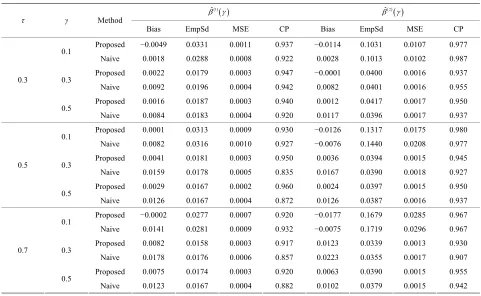
Table 2. Finite-sample for ting nti ssion ete mo with n co 1
mulation ru ach with a ple size 10
results estima the qua le regre param rs under del (8) Clayto pula. ˆ
ˆ 2
τ γ Method
Bias EmpSd MSE CP Bias EmpSd MSE CP
Proposed −0.0025 0.0330 0.0011 0.922 −0.0094 0.1261 0.0160 0.957
0.1
P 0.3
0.0005 0.927 0.0042 0.0584 0.0034 0.940
Proposed 0.0004 0.0201 0.0004 0.920 0.0001 0.0442 0.0019 0.942
0.3
Proposed −0.0015 0.0326 0010 0.925 −0.0133 0.1291 0.960
0. 0. 0. 0. 0.
0.5
− −
−
Naive 0.0032 0.0270 0.0007 0.957 −0.0076 0.1252 0.0157 0.965
roposed 0.0002 0.0194 0.0003 0.942 0.0005 0.0415 0.0017 0.932
Naive 0.0071 0.0210
0.5
Naive 0.0058 0.0199 0.0004 0.877 0.0070 0.0444 0.0020 0.915
0. 0.0168
0.1
Naive 0030 0.0288 0008 952 0011 0.1060 0.0112 977
Proposed 0.0028 0.0196 0.0003 0.912 −0.0007 0.0425 0.0018 0.913
0.3
Naive 0.0129 0.0189 0.0005 0.880 0.0098 0.0437 0.0020 0.915
Proposed 0.0010 0.0199 0.0004 0.917 0.0001 0.0418 0.0017 0.935
0.5
Naive 0.0098 0.0183 0.0004 0.891 0.0104 0.0387 0.0016 0.935
Proposed 0.0011 0.0331 0.0011 0.927 0.0087 0.1293 0.0167 0.957
0.1
Naive 0.0086 0.0264 0.0007 0.952 0.0103 0.1655 0.0275 0.942
Proposed 0.0022 0.0166 0.0002 0.942 0.0032 0.0383 0.0014 0.932
0.3
Naive 0.0166 0.0178 0.0005 0.877 0.0169 0.0413 0.0019 0.912
Proposed 0.0022 0.0180 0.0003 0.917 0.0007 0.0367 0.0013 0.957
0.7
0.5
Naive 0.0122 0.0174 0.0004 0.867 0.0108 0.0366 0.0014 0.932
[image:6.595.58.539.431.726.2]Table 3. Finite-sam fo atin ant ssio mete r m wit cop 1
ple results r estim g the qu ile regre n para rs unde odel (7) h Frank ula.
ˆ
ˆ 2
τ γ Method
Bias EmpSd MSE CP Bias EmpSd MSE CP
Proposed 0.0077 0.0316 0.0010 0.937 0.0021 0.0428 0.0018 0.947
0.1
Naive 0.0230 0.0314 0.0015 0.887 −
−
Proposed 0.0001 0.0380 0.0014 0.957 −0.0005 0.0519 0.0027 0.947
0.3
Proposed 0.0109 0.0324 0.0011 0.932 −0.0014 0.0438 0.0019 0.935
0.0104 0.0411 0.0017 0.942
Proposed 0.0045 0.0366 0.0013 0.945 0.0003 0.0517 0.0026 0.955
0.3
Naive 0.0272 0.0376 0.0021 0.892 0.0155 0.0500 0.0027 0.930
0.5
Naive 0.0203 0.0361 0.0017 0.932 −0.0127 0.0501 0.0026 0.930
0.1
0.0399 0.0325 0026 0.770 −0.0213 0.0443 0.925
Proposed 0 0 − 0
0.3
P 0.5
0.5
P
Naive 0. 0.0024
.0073 0.0388 0.0015 .937 0.0022 0.0524 0.0027 .942
Naive 0.0429 0.0360 0.0031 0.790 −0.0233 0.0507 0.0031 0.930
roposed 0.0050 0.0366 0.0013 0.947 −0.0033 0.0515 0.0026 0.962
Naive 0.0296 0.0343 0.0020 0.852 −0.0171 0.0484 0.0026 0.952
roposed 0.0261 0.0309 0.0016 0.885 −0.0130 0.0426 0.0019 0.937
0.1
P 0.3
P 0.7
0.5
Naive 0.0586 0.0325 0.0044 0.572 −0.0311 0.0443 0.0029 0.907
roposed 0.0331 0.0323 0.0021 0.867 −0.0236 0.0452 0.0026 0.915
Naive 0.0575 0.0329 0.0043 0.582 −0.0362 0.0449 0.0033 0.862
roposed 0.0210 0.0361 0.0017 0.902 −0.0158 0.0533 0.0030 0.947
Naive 0.0312 0.0341 0.0021 0.830 −0.0195 0.0512 0.0030 0.955
The results are based on 400 sim uns ea sam 0.
Table 4. Fi samp ts fo atin ant ssio met m wit cop 1
ulation r ch with a ple size 10
nite- le resul r estim g the qu ile regre n para ers under odel (8) h Frank ula.
ˆ
ˆ 2
τ γ Method
Bias EmpSd MSE CP Bias EmpSd MSE CP
Proposed −0.0049 0.0331 0.0011 0.937 −0.0114 0.1031 0.0107 0.977
0.1
Naive 0.0018 0.0288 0.0008 0.922 0.0028 0.1013 0.0102 0.987
Proposed 0.0022 0.0179 0.0003 0.947 −0.0001 0.0400 0.0016 0.937
0.3
Naive 0.0092 0.0196 0.0004 0.942 0.0082 0.0401 0.0016 0.955
Proposed 0.0016 0.0187 0.0003 0.940 0.0012 0.0417 0.0017 0.950
0.3
0.5
Proposed 0.0001 0.0313 0.0009 0.930 −0.0126 0.1317 0.0175 0.980
Naive 0.0084 0.0183 0.0004 0.920 0.0117 0.0396 0.0017 0.937
0.1
0.0082 0.0316 0.0010 0.927 −0.0076 0.1440 0.0208 0.977
Proposed 0 0 0 0
0.3
P 0.5
0.5
P
Naive
.0041 0.0181 0.0003 .950 .0036 0.0394 0.0015 .945
Naive 0.0159 0.0178 0.0005 0.835 0.0167 0.0390 0.0018 0.927
roposed 0.0029 0.0167 0.0002 0.960 0.0024 0.0397 0.0015 0.950
Naive 0.0126 0.0167 0.0004 0.872 0.0126 0.0387 0.0016 0.937
roposed −0.0002 0.0277 0.0007 0.920 −0.0177 0.1679 0.0285 0.967
0.1
P 0.3
P 0.5
Naive 0.0141 0.0281 0.0009 0.932 −0.0075 0.1719 0.0296 0.967
roposed 0.0082 0.0158 0.0003 0.917 0.0123 0.0339 0.0013 0.930
Naive 0.0178 0.0176 0.0006 0.857 0.0223 0.0355 0.0017 0.907
roposed 0.0075 0.0174 0.0003 0.920 0.0063 0.0390 0.0015 0.955
0.7
Naive 0.0123 0.0167 0.0004 0.882 0.0102 0.0379 0.0015 0.942
The results are based on 400 sim uns ea sam 0.
ulation r ch with a ple size 10
[image:7.595.57.538.429.725.2]point estimator,
1ˆ j 1
i i
j
;
the empirical st rd d ,
400
400 0 , ,2 , (Bias)j
anda eviation
400
ˆ j j
i i
2 ,=1
399
where
400
=1ˆ 0
j
i
, Sd); eansquared error, Bias2 + Em , (M d the c ge 40
j i
(Emp the m pSd2 SE); an overa probability of the 95% confidence intervals,
4000 =1
j i
I
ˆ j 1.96 j 400i Sdi ,
where j i
Sd is the estimated s
tandard deviation ofi
ˆ j
by the bootstrap approach, (CP). From the re- sults, we can see that our proposed estim or has much smaller bias and smaller mean squared error than the naive estimator. The confidence intervals coverage
se to the nom
0
at
probabilities are clo inal level 95% in most cases while the naive estimator has the coverage rate far below the nominal level in many cases. Although the proposed estimator of 1 has the coverage rate lower than 90 case with Kendall’s tau τ = 0 but it still performs better than the naive estimator. As the
d h he c e p ties opo ti-
ator e c the al l hile t v-
rage bili e n tim t wo is
nfirm at ou at ile th aive esti r is not.
The ex the sed l diagnostic
etho th od nera m
te ere), t overag robabili for pr sed es m becom lose to nomin evel w he co e proba ties for th aive es ator ge rse. Th co
wh
s th e n
r estim mato
or is asymptotically correct n we amine propo mode
m d when e true m el is ge ted fro
0
log T Z ,
here
w 0
1, Z 1 Ber
0.5
, and% in the first .7
sample size increases to n = 200 for that case (data omit-
0.5 , 0.5 0.5
U
so that
0 and
,D
follow Clayton copula with Dexp 2
. We consider τ = 0.3, 0.5, 0.7 and γ= 0.1, 0.3, 0.5 under n = 100 based on 200 replications.Three forms of transformation are fitted: 1)
t log
t ; 2) [image:8.595.58.538.424.705.2]h h t
t; 3) h t
2
t1 21
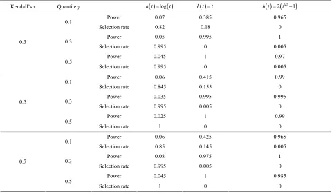
.Table 5 presents the rejection probability
200I T
n i, Z2
=1
200
i
, α = 0.05, and he probability th odel
ted as the o which gives th lest value of
where t at the fitted m
is selec ne e smal
n
T among the three candidates. From the results, we see that when h t
log
t , ion probability (type-I error rate) is close to the specified level of α = 0.05. When the fitted model is wrong, the rejection prthe reject
ost cases.
e proposed mode ecking meth .
obability (power of the test) is very high in m
l ch od
Table 5. Finite-sample results for th
Kendall’s τ Quantile γ h t log t h t t h t 2
t1 21
Power 0.07 0.385 0.965
0.1
Selection rate 0.82
Power 0.05 0.3
Selection rate 0.99
Power 0.04 0.3
0.5
Selection rate 0.995
Power 0.06 5
5
0.415 0.99
0.18 0
0.995 1
0 0.005
1 0.97
0 0.005
0.1
Selection rate 0.845 0.155 0
Power 0.035 0.995 0.995
Selection rate 0.995 0.005 0
0. 0.3
Power 0.025 1 0.99
0.5
0.5
Selection rate 1 0 0
Power 0.06 0.425 965
0.1
Selection rate 0.85 0.
0. 0. 5 0.7
145 0.005
Power 0.08 975 1
0.3
Selection rate 0.995 00 0
Power 0.045 1 0.985
0.5
Selection rate 1 0 0
Note: The sample size is 100 and replications are 200. “Power” = 200
2
1200
i
I
, wh 0.05. “Selection rate” is the oportion that the fitted model is selected as the one giving the smallest value of,
n i
T Z ere pr
n
Even for the case whe the power latively lo
around 40% (the γ = t
re 0.1
is re w
quantile for h t
), the probabilities of selecting th e still high5. Data Analysis
We app he proposed hodolog he bo marrow transplant data based on 1 a patient provided by [1]. Patie ere classi ri categories: ALL, AML low-risk, high-risk
The = 0), hig
time. S e correct model ar .
ly t met y to analyze t 37 leukemi
ne s nts w fied into three sk
and AML based on their status at the time of transplantation. covariates (Z1, Z2) are coded as ALL (Z1 = 1, Z2
ML low-risk (Z1 = 1, Z2= 0), and AML h-risk (Z1 = A
0, Z2= 1). We want to investigate how the risk classifica- tion is related to the quantile of the relapse pecifi- cally the fitted model is given by
log T Z Z1, 2
0
1
Z1 2
Z2. (9)
The results are summarized in the Tables 6 and 7 based on B = 1000 bootstrap replications. Table 6 contains the estimators and model checking tests with
21, 2 1 1 2 0.2
q Z Z Z Z . The p-value is the testing
result by the model checking approach provided in Sub- Section 3.3. Since all the p-values are greater than 0.05, we adopt the model in (9) for further analysis.
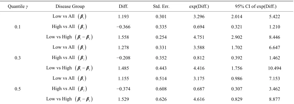
From the analysis we see that patients of AML low- risk had longer relapse time than those in the other two groups and the difference is more obvious for those with
earlier rela e. For example, the 10 antile of the re- lapse time e AML low-risk grou 964 times of that in A oup and 4.751 times t in AML high- risk grou e group differences a
nificant 10% and 30% qua but no longer significa e 50% quantile.
6. Concluding Remarks
In this pap we consider quantile reg ssion analysis for analy failur
the sem peting ris
umption is adopted to specify the dependency be-
[image:9.595.53.537.445.536.2]r variance estimation. For checking the adequacy of the fitted model, a model d. Simulation results con-
Table 6. Estimation of quantile regression parameters od
ps % qu
in th p is 3.2
LL gr of tha
p. Th for the
re statistically sig- ntiles.
nt for th
er, re
zing the e-time of a non-terminal event under i-com ks setting. The Archimedean cop- ula ass
tween the two correlated events. This assumption is util- ized to calculate the weight for bias correction in the es- timation of quantile regression parameters. Here we fo- cus on the case of discrete covariates and derive the as- ymptotic properties of the proposed estimators. The bootstrap method is suggested fo
diagnostic approach is propose
firm that the proposed methods have good performances in finite samples. In the data analysis, we see that the risk classification is particularly influential for earlier relapse. The methodology can be extended to allow for continu- ous covariates by employing some smoothing techniques but the corresponding theoretical analysis is beyond the scope of the paper.
el checking test based on the bone marrow transplant data. and m
0
β β1 β2
Quantile γ
0
ˆ
β Sd 95% CI βˆ1 Sd 95% CI βˆ2 Sd 95% CI
p-value
0.1 4.587 0.262 4.109 5.080 1.193 0.301 0.700 1.691 −0.366 0.335 −1.137 0.191 0.581
0.3 5.571 0.198 5.222 6.169 1.278 0.331
0.5 6.129 0.409 5.498 6.819 1
0.532 1.894 −0.208 0.353 −0.936 0.380 0.897
−0.014 1.968 −0.374 0.608 −1.180 1.242 0.220
.155 0.514
ela
Quantile γ Disease Group Diff. Std. Err. exp(Diff.) 95% CI of exp(Diff.)
Table 7. Comparison of leukemia r pse time for the three risk groups.
Low vs All β1 1.193 0.301 3.296 2.014 5.422
High vs All β2 −0.366 0.335 0.694 0. 21 1.210
0.1
Low vs High
3
β1β2 1. 58 0.254 4.751 2.902 8.446
s A
5
Low v ll β1 8 1. 6.647
s A
1.27 0.331 3.588 702
High v ll β2 08 0. 1.462
L ig
−0.2 0.352 0.812 392
0.3
ow vs H h β1β2 1.485 1. 494
Low vs All
0.443 4.416 756 10.
1
β 1.155 0.514 3.175 0.986 7.153
High vs All β2 −0.374 0.608 0.687 0.307 3.462
0.5
Low vs High β1β2 1.529 0.626 4.616 829 8.8770.
[image:9.595.58.538.563.734.2]
7. Acknowledgem
This r was fin ppo by the National Science Council o SC100 18-M- - MY2).
R
[1] J. P. Klein and chberger Surviva sis: Techniques for Censored and Truncated Data, Edi- tion, Springer, New York, 2003.
[2] J. Powell, “Least eviations Estimat e Censored Regression Model,” Jour l of Eco rics,
5.
4)90004-6
ent
pape ancially su rted
f Taiwan (N -21 194-003
EFERENCES
M. L. Moes , “ l Analy ” 2nd Absolute D ion for th
na nomet
[ . Peng and Fine, “Co g Risks Q Re- gression,” Journal of the American Statistical Association,
ol. 104, N 2009, pp. 453.
i:10.1198 009.tm082
Vol. 25, No. 3, 1984, pp. 303-32
doi:10.1016/0304-4076(8
[3] J. Powell, “Censored Regression Qunatiles,” Journal of Econometrics, Vol. 32, No. 1, 1986, pp. 143-155.
doi:10.1016/0304-4076(86)90016-3
[4] B. Fitzenberger, “A Guide to Censored Quantile Re sions,” In: G. S. Maddala and C. R. Rao, Eds.,
books of Statis sterdam, 1997, pp
405-437. doi:10.1016/S0169-7161(97)15017-9
gres-
Hand-
.
tics, North-Holland, Am
307/2998578
[5] M. Buchinsky and J. Hahn, “A Alternative Estimator for Censored Quantile Regression,” Econometrica, Vol. 66, No. 3, 1998, pp. 653-671. doi:10.2
, No. 429, 1995, pp.
.10476500
[6] Z. Ying, S. H. Jung and L. J. Wei, “Survival Analysis with Median Regression Models,” Journal of the Ameri- can Statistical Association, Vol. 90
178-184. doi:10.1080/01621459.1995
l
l. 94, No. 445, 1999, [7] S. Yang, “Censored Median Regression Using Weighted
Empirical Survival and Hazard Functions,” Journa American Statistical Association,Vo
of the
pp. 137-145. doi:10.1080/01621459.1999.10473830
[8] S. Portnoy, “Censored Regression Quantiles,” Journal of the American Statistical Association, Vol. 98, No. 464, 2003, pp. 1001-1012. doi:10.1198/016214503000000954
pp. 637-[9] L. Peng and Y. Huang, “Survival Analysis Based on
Quantile Regression Models,” Journal of the American Statistical Association, Vol. 103, No. 482, 2008,
649. doi:10.1198/016214508000000355
[10] G. Yin, D. Zeng and H. Li, “Power Transformed Linear Quantile Regression with Censored Data,” Journal of the American Statistical Association, Vol. 103, No. 483, 2008, pp. 1214-1224. doi:10.1198/016214508000000490
[11] S. Portnoy and G. Lin, “Asymptotics for Censored Re- gression Quantiles,” Journal of Nonparametric Statistics, Vol. 22, No. 1, 2010, pp. 115-130.
doi:10.1080/10485250903105009
[12] J. P. Fine, H. Jiang and R. Chappell, “On Semi-Compet- ing Risks Data,” Biometrika, Vol. 88, No. 4, 2001, pp. 907-919.
13] L J. P. mpetin uantile
V o. 488, 1440-1
do /jasa.2 28
[14] R. Li and L. Peng, “Quantile Regression for Left-Trun- ted Semi ing Risks Biometri l. 67 o. 3, 2011 1-710.
/j.15
ca compet Data,” cs, Vo
N , pp. 70
41-0420.2010.0
doi:10.1111 1521.x
[ . J. Patton eling Asy ic Exchan De- ndence,” tional Eco Review,V , No.
, pp. 527
i:10.1111 -2354.200 7.x
15] A , “Mod mmetr ge Rate
pe 2, 2006
Interna
-556.
nomic ol. 47
do /j.1468 6.0038
[ . Wang, ating the Association Pa r for
enden ,”
o. 1, 16] W
Copula Models “Estimunder Dep t Censoring ramete Journal of the Royal Statistical Society, Series B, Vol. 65, N 2003, pp. 257-273. doi:10.1111/1467-9868.00385
[17] L. Lakhal, L.-P. Rivest and B. Abdous, “Estimating Sur-vival and Association in a Semicom
Biometrics, Vol. 64, No. 1, 2008, p
peting Risks Model,” p. 180-188.
doi:10.1111/j.1541-0420.2007.00872.x
[18] M. Fygenson and Y. Ritov, “Monotone Estimating Equa- tions for Censored Data,” The Annals of Statistics,Vol. 22, No. 2, 1994, pp. 732-746.
doi:10.1214/aos/1176325493
[19] L.-P. Rivest and M. Wells, “A Martinga the Copula-Graphic Estimator fo
le Approach to r the Survival Function under Dependent Censoring,” Journal of Multivariate Analysis, Vol. 79, No. 1, 2001, pp. 138-155.
doi:10.1006/jmva.2000.1959
[20] J. X. Zheng, “A Consistent Nonparametric Regression Models under Quantile Restrictions,” Econometric The- ory,Vol. 14, No. 1, 1998, pp. 123-138.
doi:10.1017/S0266466698141051
[21] J. L. Horowitz and V. G. Spokoiny, “An Adaptive, Rate- Optimal Test of Linearity for Median Regression Mod- els,” Journal of the American Statistical Association, Vol. 97, No. 459, 2002, pp. 822-835.
doi:10.1198/016214502388618627
[22] X. He and L. Zhu, “A Lack-of-Fit Test for Quantile Re- gression,” Journal of the American Statistical Association, Vol. 98, No. 464, 2003, pp. 1013-1022.
doi:10.1198/016214503000000963
[23] D. Y. Lin and L. J. Wei and Z. Ying, “Checking the Cox Model with Cumulative Sums of Martingle-Based Resi- duals,” Biometrika, Vol. 80, No. 3, 1993, pp. 557-572.
doi:10.1093/biomet/80.3.557
[24] R. Braekers and N. Veraverbeke, “A Copula-Graphic Es- timator for the Conditional Survival Function under De- pendent Censoring,” The Canadian Journal of Statistics, Vol. 33, No. 3, 2005, pp. 429-447.