D S Sharma, R Sangal and J D Pawar. Proc. of the 11th Intl. Conference on Natural Language Processing, pages 277–286, Goa, India. December 2014. c2014 NLP Association of India (NLPAI)
Manipuri Chunking:
An Incremental Model with POS and RMWE
Kishorjit Nongmeikapam1,
Thiyam Ibungomacha Singh2, Ngariyanbam Mayekleima Chanu3, Sivaji Bandyopadhyay4
1,2
Deptt. of Computer Science and Engg., MIT Manipur University, Imphal, India [email protected]
3
Deptt. of Education, Govt. of Manipur, India [email protected]
4
Deptt. of Computer Science and Engg. Jadavpur University, Kolkata, India
Abstract
This paper records the work of Manipuri Chunking by using the commonly use tool of Support Vector Machine (SVM). Manipur being a very highly agglutinative language have to be careful in selecting the features for running the SVM. An experiment is being performed with 35,000 words to check whether the POS tagged
and the Reduplicated Multiword
Expression (RMWE) can improve the Chunk identification. With a linguistic expert the Newspaper corpus is maintained to the Gold standard. The experimental system is designed as an incremental model with notation and identification in each stage. The Chunks are identified with a list of selected features. The chunks are very much related with the Part of Speech (POS) thus in the second stage POS tagging is done with the identified Chunks as one of the features which is again followed by the chunking. The third stage is with the RMWE. An experiment is again conducted with a list of carefully selected features for the SVM in order to find the Chunk with POS and RMWE as other features. Comparisons and evaluations are performed in each phase and the final
output is drawn with completely tagged chunk Manipuri text. The experiment also identifies the POS tagging with a Recall (R) of 71.97%, Precision (P) of 87.16% and F-measure (F) of 78.84%. Apart from POS it also identifies the RMWE with a Recall (R) of 89.39%, Precision (P) of 98.33% and F-measure (F) of 93.65%. The system shows a final chunking with a Recall (R) of 70.45%, Precision (P) of 86.11% and F-measure (F) of 77.50%.
Keywords-SVM; POS; Chunk; RMWE; Manipuri
1. INTRODUCTION
Chunking is the process of identifying and labeling the simple phrases (it may be a Noun Phrase or a Verb Phrase) from the tagged output, of which the utterance of words for a given phrase forms as a chunk for this language [1]. The POS and RMWE might also play an important role in the SVM-based Manipuri chunking.
The present work of chunking is done in order to come up with a reliable chunking system for this under privilege Language. Manipuri language is a schedule Indian language widely spoken in the state Manipur, a North-Eastern part of India, and in the countries of Myanmar and Bangladesh. The Manipuri
Language belongs to the Tibeto-Burman type of language and is a high agglutinative class of language.
The work reported here consists of a multi stage identification or incremental model of the Chunks. The first output is a chunk file which is followed by the POS then again a chunk tagged file. The RMWE is identified in the next incremental stage which is again followed by a Manipuri chunked file. The final output being the SVM based Manipuri chunk with POS and RMWE as one among the selected features.
The paper is arranged in such a way that the related works is listed in Section 2. Section 3 writes about the Reduplicated Multiword Expression (RMWE) which is followed by the Manipuri agglutinative explanation at Section 4. Section 5 describes the concept of Support Vector Machine (SVM) which is followed by the System design at 6. The experiment and evaluation is discussed at Section 7 and the conclusion is drawn at Section 8.
2.RELATED WORKS
Works on chunking are reported in [2] using Maximum Entropy Model. Apart from the above approaches, the CRF based chunking utilizes and gives the best of the generative and classification models. It resembles the classical model, in a way that they can accommodate many statistically correlated features of the inputs. And consecutively, it resembles the generative model, they have the ability to trade-off decisions at different sequence positions, and consequently it obtains a globally optimal labeling. It is shown in [3]-[4] that CRFs are better than related classification models. Parsing by chunks is discussed in [5]. Dynamic programming for parsing and estimation of stochastic unification-based grammars is mentioned in [6] and other related works are found in [7]-[9].
Manipuri Chunking using with CRF is reported in [1]. Until now, no works of SVM based chunking has ever been reported for the Manipuri language. Most of the previous works for other languages on this area make use of two machine-learning approaches for sequence labeling, namely CRF and the second approach as the sequence labeling problem as a sequence of a classification problem, one for each of the labels in the sequence.
The works on chunking can be observed applying both rule based and the probabilistic or statistical methods and for the Manipuri text chunking, the paper in [1] proposed a Conditional Random Field based approach.
3.REDUPLICATED MWE
Manipuri is a tonal language and Reduplicated Multiword Expressions are abundant. Work of RMWE identification Works for Manipuri is reported in [10] and using CRF in [11]. Reduplicated Multiword Expression is as defined in [12] as: ‘reduplication is that repetition, the result of which constitutes a unit word’. The Classification for reduplicated MWEs in Manipuri mention in [12] is as follows: 1) Complete Reduplicated MWEs, 2) Mimic Reduplicated MWEs, 3) Echo Reduplicated MWEs and 4) Partial Reduplicated MWEs. Apart from these fours there are also cases of a) Double reduplicated MWEs and b) Semantic Reduplicated MWEs.
3.1 Complete Reduplicated MWEs
The single word or clause is repeated once forming a single unit regardless of phonological or morphological variations in the complete Reduplication MWEs. In the Manipuri Language these complete reduplication MWEs can occur as Noun, Adjective, Adverb,
Wh-question type, Verbs, Command and Request. For example, (‘mǝrik mǝrik’)which means ‘drop by drop’.
3.2 Partial Reduplicated MWEs
The second word carries some part of the first word as an affix to the second word, either as a suffix or a prefix for the partial reduplication. For example, ( ‘cǝt-thok cǝ t-sin’) means ‘to go to and fro’, ( ‘sa-mi lan-mi’) means ‘army’.
3.3 Echo Reduplicated MWEs
In the Echo RMWE the second word does not have a lexicon semantics and is basically an echo word of the first word. For example, thk-si
kha-si means ‘good manner’. Here the first
word has a dictionary meaning ‘good manner´
but the second word does not have a dictionary meaning and is an echo of the first word.
3.4 Mimic Reduplicated MWEs
The words are complete reduplication but the morphemes are onomatopoetic, usually emotional or natural sounds in the mimic RMWE. For example, (‘khrǝk khrǝk’) means ‘cracking sound of earth in drought’.
3.5 Double Reduplicated MWEs
The double Reduplicated MWE consists of three words, where the prefix or suffix of the first two words is reduplicated but in the third word the prefix or suffix is absent. An example of double prefix reduplication is i i
(‘i-mun i-mun mun-ba’) which means,
‘completely ripe’. It may be noted that the prefix is duplicated in the first two words while in the following example suffix reduplication take place, (‘ƞǝω-srok ƞǝω -srok ƞǝω-ba’)which means ‘shining white’.
3.6 Semantic Reduplicated MWEs
In the case of Semantic RMWE, both the reduplication words have the same meaning as well as the MWE. Such type of MWEs is very special to the Manipuri language. For example,
(‘pamba kǝy’ ) means ‘tiger’ and each
of the component words means ‘tiger’.
Semantic reduplication exists in Manipuri in abundance as such words have been generated from similar words used by seven clans in Manipur during the evolution of the language.
4. MANIPURI AGGLUTINATIVENESS AND STEMMING
As in mention in [13] altogether 72 (seventy two) affixes are listed in Manipuri out of which 11 (eleven) are prefixes and 61 (sixty one) are suffixes. Table I shows the prefixes of 10 (ten number) because the prefix (mə) is used as formative and pronomial so only one is included and like the same way Table II shows the suffixes in Manipuri with only are 55 (fifty five) suffix in the table since some of the suffixes are used with different form of usage such as
(gum) which is used as particle as well as proposal negative, (də) as particle as well as locative and (nə) as nominative, adverbial, instrumental or reciprocal.
To prove with the point that Manipuri is highly agglutinative let us site an example word:
“я ”
(“pusinhənjərəmgədəbənidəko”), which means “(I wish I) myself would have caused to bring in (the article)”. Here there are 10 (ten) suffixes being used in a verbal root, they are “pu” is the verbal root which means “to carry”, “sin”(in or inside), “hən” (causative), “jə”
(reflexive), “rəm” (perfective), “gə”
(associative), “də” (particle), “bə”
(infinitive), “ni” (copula), “də”
(particle) and “ko” (endearment or wish).
TABLE I. PREFIXES IN MANIPURI
TABLE II. SUFFIXES IN MANIPURI
The stemming of Manipuri words are stemmed by stripping the suffixes in an iterative manner as mention in [13]. As mention in above a Manipuri word is rich of suffixes and prefixes. In order to stem a word an iterative method of stripping is done by using the acceptable list of prefixes (11 numbers) and suffixes (61 numbers) as mention in table 1 and table 2 above.
5. CONCEPT OF SUPPORT VECTOR MACHINES (SVM)
The idea of Support vector machines (SVM) were first shared by Vapnik [14]. In the work of
Prefixes used in Manipuri
a, i, i, @, , A, , , and
Suffixes used in Manipuri
, k, , @, @, @ i, @, @ C, , , , , , , , , , , , , , , , , t, , E, , , , F , , , , , , , , , , l, , , H, , , , C, , , E, , I, and
[15] it is mention that Support Vector Machines is one of the new techniques for pattern classification which have been widely used in many application areas. The kernel parameters setting for SVM in training process impacts on the classification accuracy. Feature selection is another factor that impacts classification accuracy.
5.1 The optimal hyperplane (linear SVM)
SVM concepts for typical two-class classification problems can be discussed for explanation. Given a training set of instance-label pairs , , = 1,2, … , where ∈ and ∈ { +1, −1}, for the linearly
separable case, the data points will be correctly classified by,
〈. 〉 + ≥ +1 = +1
(1)
〈. 〉 + ≤ +1 = −1 (2)
Combining Eqs. (1) and (2) into one set of inequalities.
〈. 〉 + − 1 ≥ 0 ∀ = 1, …
(3)
The SVM finds an optimal separating hyperplane with the maximum margin by solving the following optimization problem: Min$,%&'( (4)
subject to: 〈. 〉 + − 1 ≥ 0
It is known that to solve this quadratic optimization problem one must find the saddle point of the Lagrange function:
)*, , + =&'(. − ∑ +-.& 〈. 〉 +
− 1 (5)
Where, the + denotes Lagrange multipliers, hence +≥ 0. The search for an optimal saddle point is necessary because the Lp must be minimized with respect to the primal variables w and b and maximized with respect to the non-negative dual variable +. By differentiating with respect to w and b, the following equations are obtained:
/
/$)*= 0, = ∑ +-.& (6)
/
/$)*= 0, ∑ +-.& = 0
(7)
The Karush Kuhn–Tucker (KTT) conditions for the optimum constrained function are necessary and sufficient for a maximum of Eq. (5). The
corresponding KKT complementarity conditions are:
+0〈. 〉 + − 11 = 0 ∀
(8)
Substitute Eqs. (6) and (7) into Eq. (5), then )* is transformed to the dual Lagrangian )2+,
Max5)2+ =
∑ +-.& −&'∑-,6.&++66〈. 6〉
(9)
subject to + ≥ 0, = 1, … , and ∑ +-.& = 0
To find the optimal hyperplane, a dual Lagrangian )2+must be maximized with respect to non-negative +. This is a standard quadratic optimization problem that can be solved by using some standard optimization programs. The solution + for the dual optimization problem determines the parameters ∗and ∗ of the optimal hyperplane. Thus, we
obtain an optimal decision hyperplane , +∗, ∗ (Eq. (10)) and an indicator decision
function sign 0, +∗, ∗1.
, +∗, ∗ = ∑
+∗〈, 〉 + ∗−
-.&
∑-∈89+∗〈. 〉 + ∗ (10)
In a typical classification task, only a small subset of the Lagrange multipliers + usually tends to be greater than zero. Geometrically, these vectors are the closest to the optimal hyperplane. The respective training vectors having nonzero + are called support vectors, as the optimal decision hyperplane , +∗, ∗ depends on them exclusively.
5.2 The optimal hyper-plane for non-separable data (linear generalized SVM)
The above concepts can also be extended to the non separable case, i.e. when Eq. (3) there is no solution. The goal is to construct a hyperplane that makes the smallest number of errors. To get a formal setting of this problem we introduce the non-negative slack variables : ≥ 0, = 1, … , . Such that
〈. 〉 + ≥ +1 − : = +1
(11)
〈. 〉 + ≤ −1 + : = −1
(12)
In terms of these slack variables, the problem of finding the hyperplane that provides the minimum number of training errors, i.e. to keep
the constraint violation as small as possible, has the formal expression:
Min$,%,;&'( + < ∑ :-.&
(13)
subject to : 〈. 〉 + + :− 1 ≥ 0, : ≥ 0
This optimization model can be solved using the Lagrangian method, which is almost equivalent to the method for solving the optimization problem in the separable case. One must maximize the same dual variables Lagrangian )2+ (Eq. (14)) as in the separable case.
Max5)2+ =
∑ +-.& −&'∑-,6.&++66〈. 6〉
(14)
subject to: 0 ≤ + ≤ <, , … , and ∑ +-.& = 0
To find the optimal hyperplane, a dual Lagrangian )2+ must be maximized with respect to non-negative + under the constrains:
∑ + = 0 =>? 0 ≤ +≤
<, = 1, … , . The penalty parameter C, which
is now the upper bound on +, is determined by the user. Finally, the optimal decision hyperplane is the same as Eq. (10).
5.3 Non-linear SVM
The nonlinear SVM maps the training samples from the input space into a higher-dimensional feature space via a mapping function , which are also called kernel function. In the dual Lagrange (9), the inner products are replaced by the kernel function (15), and the non-linear SVM dual Lagrangian )2+ (Eq. (16)) is similar with that in the linear generalized case.
@Φ.ΦA6BC ≔ E6
(15)
)2+ = ∑ +-.& −&'∑-,6.&++66E〈. 6〉
(16)
subject to: 0 ≤ + ≤ <, = 1, … , and ∑ +-.& = 0
This optimization model can be solved using the method for solving the optimization in the separable case. Therefore, the optimal hyperplane has the form Eq. (17). Depending upon the applied kernel, the bias b can be implicitly part of the kernel function. Therefore, if a bias term can be accommodated within the
kernel function, the nonlinear SV classifier can be shown as Eq. (18).
, +∗, ∗ = ∑ +
∗
-.& 〈Φ.ΦA6B〉 + ∗. = ∑ -.& +∗E, + ∗
(17)
, +∗, ∗ = ∑
+∗
∈89 〈Φ,ΦA6B〉. = ∑∈89+∗E,
(18)
Some kernel functions include polynomial, radial basis function (RBF) and sigmoid kernel, which are shown as functions (19), (20), and (21). In order to improve classification accuracy, these kernel parameters in the kernel functions should be properly set.
Polynomial kernel: EA, 6B = A1 + 6BF
(19)
Radial basis function kernel:
EA, 6B = GH @−IJ− 6J'C
(20) Sigmoid kernel:
EA, 6B = K=>ℎAE. 6− MB
(21)
6. WORKING OF THE SYSTEM
The experimental set up of the system uses SVM. The running of the training process has been carried out by YamCha1 toolkit, an SVM based tool for detecting classes in documents and formulating the tagging task of Chunking, POS and RMWE as a sequential labelling problem. Here, the pairwise multi-class decision method and polynomial kernel function have been used. For classification, TinySVM-0.072 classifier is used which is readily available as open source for segmenting or labeling sequential data.
A list of possible features is prepared. The listed features are tried with different combinations in order to come up with the best possible Chunk. The best output Chunk is evaluated with the best features combinations. The features are again used for the SVM based POS tagging with the identified Chunk. The words are now tag with the POS. This POS is used as another feature for the chunking. This is
1http://chasen-org/~taku/software/yamcha/
2http://chasen-org/~taku/software/TinySVM/
done because chunking is very much related with POS.
Manipuri generally is a tonal language and is abundant with the RMWEs. RMWEs are identified using the SVM with features selected including POS and the identified Chunk. These identified RMWEs are used again for the identification of final Chunks in the text file. Fig.1 explains the System block diagram.
The Chunk tag is the I-O-B tagging as shown in Table III:
TABLE III. IOBCHUNK TAGGING
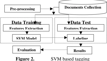
[image:6.612.318.537.30.156.2]The processing and running of the SVM is shown on Fig. 2.
Figure 1. System Block diagram
The input file for the first time is a training file which gives an output in the form of a model file and in the second run the input file is a testing file. The output file after running the SVM on the input testing file is a labeled file.
Figure 2. SVM based tagging
The working of SVM is mainly based on the feature selection. The feature listed for the Chunk tagging is as follows:
F= { Wi-m, … ,W i-1, W i, W i+1, …, W i+n, SWi-m,
…, SWi-1, SWi, SWi+1,… , SWi-n , number of
acceptable standard suffixes, number of acceptable standard prefixes, acceptable suffixes present in the word, acceptable prefixes present in the word, word length, word frequency, digit feature, symbol feature}
The details of the set of features that have been applied for Chunking in Manipuri text are as follows:
1. Surrounding words as feature: Preceeding word(s) or the successive word(s) are important in Chunking because these words play an important role in determining the Chunk of the present word.
2. Surrounding Stem words as feature: The Stemming algorithm mentioned in [13] is used. The preceding and the following stemmed words of a particular word can be used as features. It is because the preceding and the following words influence the present word Chunk.
3. Number of acceptable standard suffixes as feature: As mention in [13], Manipuri being an agglutinative language the suffixes plays an important in determining the Chunk of a word. For every word the number of suffixes are identified during stemming and the number of suffixes is used as a feature.
4. Number of acceptable standard prefixes as feature: Prefixes plays an important role for Manipuri language. Prefixes are identified during stemming and the prefixes are used as a feature.
B-X Beginning of the chunk word X
I-X Intermediate or non beginning chunk word X
O Word outside of the chunk text
Evaluation Results
Pre-processing Documents Collection
Data Test
Labeling Features Extraction Data Training
SVM Model Features Extraction
CHUNK
TEX T FILE
POS TAGGING
CHUNK MWE
IDENTIFICATI ON
CHUNK
[image:6.612.88.294.329.601.2]5. Acceptable suffixes present as feature: The standard 61 suffixes of Manipuri which are identified is used as one feature. The maximum number of appended suffixes is reported as ten. So taking into account of such cases, for every word ten columns separated by a space are created for every suffix present in the word. A “0” notation is being used in those columns when the word consists of no acceptable suffixes.
6. Acceptable prefixes present as feature: 11 prefixes have been manually identified in Manipuri and the list of prefixes is used as one feature. For every word if the prefix is present then a column is created mentioning the prefix, otherwise the “0” notation is used.
7. Length of the word: Length of the word is set to 1 if it is greater than 3 otherwise, it is set to 0. Very short words are generally pronouns and rarely proper nouns.
8. Word frequency: A range of frequency for words in the training corpus is set: those words with frequency <100 occurrences are set the value 0, those words which occurs >=100 are set to 1. It is considered as one feature since occurrence of determiners, conjunctions and pronouns are abundant.
9. Digit features: Quantity measurement, date and monetary values are generally digits. Thus the digit feature is an important feature. A binary notation of ‘1’ is used if the word consist of a digit else ‘0’.
10. Symbol feature: Symbols like $,% etc. are meaningful in textual use, so the feature is set to 1 if it is found in the token, otherwise 0. This helps to recognize Symbols and Quantifier number tags.
7.EXPERIMENT AND EVALUATION
The text document file collected from a Newspaper domain is cleaned for processing where the error and grammatical mistakes are minutely checked by a linguist. For the Chunking the expert also marks each word with the IOB format of Chunk. The marked Chunk texts are used for both training and testing.
Apart from the above IOB-Chunk marking the expert is asked to identify the POS and RMWE for the use in training and testing of the system.
The system used approximately 35000 words corpus for the training and testing. This corpus
is considered as gold standard since an expert manually identifies the required Chunk, POS and RMWE words. Fig.3 shows the sample of POS and chunking which are marked by the expert.
………. ...
o NN B-X
a JJ B-X
NC I-X
a QT I-X
VFC B-X
| SYM O ………. ………..
Figure 3. Sample of the words with POS and BOI chunking
Of the 35000 words 25000 words are considered for the training and the rest of the 10000 are used for the testing.
Evaluation is done with the parameter of Recall, Precision and F-score as follows:
Recall, R =
text the in ans correct of No
system the by given ans correct of No
Precision, P =
system the by given ans of No
system the by given ans correct of No
F-score, F =
R R R R P P P P 2222 ββββ
1)PR 1)PR 1)PR 1)PR 2222
( ( ( (ββββ
+ +
Where ββββ is one, precision and recall are given equal weight.
7.1 Chunking using SVM
The first step of the identifying the chunks are performed using SVM. As mention in Section 6, the feature list is identified and performs the experiment with different combinations.
TABLE IV. MEANING OF THE NOTATIONS
TABLE V. SYSTEM PERFORMANCE WITH
VARIOUS FEATURE COMBINATIONS FOR CHUNK IDENTIFICATION
The Table no V shows some of the best combinations of the results with Table no IV showing the explanations of the symbols used. The best combination for the chunking after performing the experiments is as follows: F= { W i-1, W i, W i+1, SWi-1, SWi, SWi+1, upto
one acceptable prefixes present in the word, upto four acceptable suffixes present in the word, word length, word frequency, number of acceptable standard suffixes, number of acceptable standard prefixes, digit feature, symbol feature}
The above feature combination shows the Recall (R) of 60.61%, Precision (P) of 79.21% and F-measure (F) of 68.67%.
7.2 SVM based POS tagging with Chunks
Similar with the experiment mention in [16] is performed in order to identify the best suitable features. Same experimental set up is used for the SVM based POS tagging. The best F-measure among the results of the SVM based POS tagging is considered the best result. This happens with the following feature set:
F= {Wi-2, W i-1, W i, W i+1, SWi-1, SWi, SWi+1,
number of acceptable standard suffixes, number of acceptable standard prefixes, acceptable suffixes present in the word, acceptable prefixes present in the word, word length, word frequency, digit feature, symbol feature}
The experimental result of the above feature combination shows the best result, which gives the Recall (R) of 71.43%, Precision (P) of 83.11% and F-measure (F) of 77.67%.
Now with the identification of the Chunk as mention in the above Section 7.2, the SVM based POS tagging is added with an extra feature in the above mention feature set. This is done in order to compare with the new set of POS tagging.
The new experimental result shows a better Recall (R) of 71.97%, Precision (P) of 87.16% and F-measure (F) of 78.84%.
7.3 SVM based Chunking with POS tag
The experiment is followed with the chunking of the system again. In this experiment the identified chunk by the SVM in the previous run is neglected instead replace with the gold standard Chunk data for training and testing. This is done so that a better result is yield. Also the previous chunking was done in order to make comparison and only to identify the POS. In the repeat of the experiment with the additional feature of POS tagging, the new feature combination becomes as follows:
F= {POS, W i-1, W i, W i+1, SWi-1, SWi, SWi+1,
upto one acceptable prefixes present in the word, upto four acceptable suffixes present in the word, word length, word frequency, number of acceptable standard suffixes, number of acceptable standard prefixes, digit feature, symbol feature}
Notation Meaning W[-i,+j] Words spanning from the ith
left position to the jth
right position
SW[-i, +j] Stem words spanning from the ith
left to the jth
right positions
P[i] The i is the number of acceptable prefixes considered
S[i] The i is the number of acceptable suffixes considered
L Word length
F Word frequency
NS Number of acceptable suffixes
NP Number of acceptable prefixes
D Digit feature (0 or 1)
SF Symbol feature (0 or 1)
Feature R(in %) P(in %) FS(in %)
W[-1,+1], SW[-1,+1], P[1],
S[4], L, F, NS, NP, D, SF 60.61 79.21 68.67
W[-2,+1], SW[-2,+1], P[1],
S[4], L, F, NS, NP, D, SF 60.61 79.21 68.67
W[-3,+1], SW[-3,+2], P[1],
S[5], L, F, NS, NP, D 62.96 61.82 62.38
W[-1,+1], SW[-1,+1], P[1],
S[4], L, F, NS, NP 50.00 82.50 62.26
W[-1,+2], SW[-2,+2], P[1],
S[4], L, F, NS, NP, D, SF 41.67 73.33 53.14
W[-4,+4], SW[-4,+4], P[3],
S[10], NS, NP 52.78 58.76 55.61
W[-1,+4], SW[-4,+1], P[2],
S[6], L, NP, SF 39.39 69.33 50.24
W[-3,+3], SW[-2,+3], P[2],
S[5], L, F, NS, SF 39.39 67.53 49.76
W[-1,+3], SW[-3,+3], P[3],
S[9], L, F, D, SF 31.25 74.47 44.03
The new experimental result shows a better Recall (R) of 61.36%, Precision (P) of 81.82% and F-measure (F) of 70.13%.
7.4 SVM based RMWE identification with Chunk and POS features
From the list of features listed in Section 6 the experiment of SVM based RMWE identification is performed. In this experimental run the Chunks and POSs are included as other features. The POS plays an important role in the identification of the RMWE also the Chunks. Like before different features combination are tried to identify the best possible combination.
* C= Chunk and **POS[-i, +j]= POS spanning from the ith
left position to the jth
right position
TABLE VI. SYSTEM PERFORMANCE WITH VARIOUS
FEATURE COMBINATIONS FOR RMWE
IDENTIFICATION
The best feature selection for SVM based RMWE identification is as follows:
F= { C, POS[-1,+1], W i-1, W i, W i+1, SWi-1,
SWi, SWi+1, upto one acceptable suffixes
present in the word, upto four acceptable prefixes present in the word, word length, word frequency, number of acceptable standard suffixes, number of acceptable standard prefixes, digit feature, symbol feature}
From the Table no VI we can observe that the best result is with the Recall (R) of 89.39%,
Precision (P) of 98.33% and F-measure (F) of 93.65%.
7.5 SVM Based Chunking after POS tagging and RMWE identification
The best result of the experiment for chunking so far without the RMWE is Recall (R) of 61.36%, Precision (P) of 81.82% and F-measure (F) of 70.13%.
The features combination was as follows:
F= {POS, W i-1, W i, W i+1, SWi-1, SWi, SWi+1,
upto one acceptable prefixes present in the word, upto four acceptable suffixes present in the word, word length, word frequency, number of acceptable standard suffixes, number of acceptable standard prefixes, digit feature, symbol feature}
After the identification of RMWE the new feature set becomes the following:
F= {RMWE, POS, W i-1, W i, W i+1, SWi-1, SWi,
SWi+1, upto one acceptable prefixes present
in the word, upto four acceptable suffixes present in the word, word length, word frequency, number of acceptable standard suffixes, number of acceptable standard prefixes, digit feature, symbol feature}
The best result for chunking with POS tagging and the Reduplicated MWEs is shown in table 7.
TABLE VII. CHUNKING RESULT WITH POS AND
RMWE
8. CONCLUSION
So far, the SVM based chunking work on Manipuri is not reported. An incremental approach is designed where the Chunking is performed at the first stage which is followed by the POS tagging, which is again followed by Chunking. With Chunk and POS as features it tagged the RMWE and Chunking is followed to find the final result.
In this experiment the POS tagging with the identified Chunks shows a Recall (R) of 71.97%, Precision (P) of 87.16% and F-measure (F) of 78.84%.
Feature R(in %) P(in %) FS(in %)
C*, POS**[-1,+1], W[-1,+1], SW[-1,+1], P[1], S[4], L, F, NS, NP, D, SF
89.39 98.33 93.65
C, POS[-1,+1], W[-2,+1], SW[-2,+1], P[1], S[4], L, F, NS, NP, D, SF
87.88 96.67 92.06
C, POS[-1,+1], W[-3,+1], SW[-3,+2], P[1], S[5], L, F, NS, NP, D
87.76 84.78 86.24
C, POS[-1,+1],W[-1,+1],
SW[-1,+1], P[1], S[4], L, F, NS, NP 82.58 90.83 86.51 C, POS[-2,+2],W[-1,+2],
SW[-2,+2], P[1], S[4], L, F, NS, NP, D, SF
78.87 76.87 77.86
C, POS[-3,+3],W[-4,+4],
SW[-4,+4], P[3], S[10], NS, NP 64.78 63.99 64.38
POS[-1,+1],W[-1,+4],
SW[-4,+1], P[2], S[6], L, NP, SF 56.82 66.96 61.48 C, W[-3,+3], SW[-2,+3], P[2],
S[5], L, F, NS, SF 50.76 59.82 54.92
W[-1,+3], SW[-3,+3], P[3],
S[9], L, F, D, SF 52.88 50.14 51.47
Model Recall Precisio
n
F-Score SVM 70.45 86.11 77.50
The RMWE identification also shows a Recall (R) of 89.39%, Precision (P) of 98.33% and F-measure (F) of 93.65%.
Comparatively, from the initial stage Chunking with a Recall (R) of 60.61%, Precision (P) of 79.21% and F-measure (F) of 68.67% the Chunking improves to a Recall (R) of 70.45%, Precision (P) of 86.11% and F-measure (F) of 77.50% with the POS and RMWE in this incremental way of Chunking experiment.
The complexity still lies with the agglutinative nature of the language. Other algorithms for the improvement of the score can also be worked on for different domains.
REFERENCES
[1] Kishorjit N,Chiranjiv Ch, Nepoleon
K,Biakchungnunga Varte and Sivaji B.,
“Chunking in Manipuri Using CRF”,
International Journal on Natural Language Computing (IJNLC) Vol. 3, No.3, June 2014, pp. 121-127.
[2] Rob Koeling, 2000, “Chunking with Maximum
Entropy Models”, Proceedings of CoNLL-2000 and LLL-2000, pp. 139-141, Lisbon, Portugal, 2000
[3] Fei Sha and Fernando Pereira,“Shallow Parsing
with Conditional Random Fields”.In the Proceedings of HLT-NAACL 2003.
[4] John Lafferty, Andrew McCallum and Fernando
Pereira, Conditional Random Fields:
Probabilistic Models for Segment-ing and Labeling Sequence Data.
[5] S. Abney. Parsing by chunks. In R. Berwick, S.
Abney, and C. Tenny, editors, Principle-based Parsing. Kluwer Academic Publishers, 1991.
[6] S. Geman and M. Johnson. Dynamic
programming for parsing and estimation of
stochastic uni_cation-based grammars. In Proc.
40th ACL, 2002.
[7] A. Ratnaparkhi. A linear observed time
statistical parser based on maximum entropy models. In C. Cardie and R. Weischedel, editors,
EMNLP-2. ACL, 1997.
[8] E. F. T. K. Sang. Memory-based shallow
parsing. Journal ofMachine Learning Research,
2:559.594, 2002.
[9] T. Zhang, F. Damerau, and D. Johnson. Text
chunking based on a generalization of winnow.
Journal of Machine Learning Research, 2:615.637, 2002.
[10] Kishorjit, N., Bandyopadhyay, S.: Identification of Reduplicated MWEs in Manipuri: A Rule
based Approached. In: Proceedings of 23rd
International Conference on the Computer Processing of Oriental Languages (ICCPOL-2010), pp 49-54, Redwood City, San Francisco, USA(2010)
[11] Kishorjit, N., Dhiraj, L., Bikramjit Singh, N., Mayekleima Chanu, Ng. & Sivaji, B., (2011)
Identification of Reduplicated Multiword Expressions Using CRF, A. Gelbukh (Ed.):CICLing 2011, LNCS vol.6608, Part I, Berlin, Germany: Springer-Verlag, pp. 41–51
[12] Singh, Ch. Y.:Manipuri Grammar, Rajesh
Publications, pp.190-204, Delhi, India (2000)
[13] Kishorjit, N., Bishworjit, S., Romina, M.,
Mayekleima Chanu, Ng. & Sivaji, B., (2011) A Light Weight Manipuri Stemmer, In the Proceedings of Natioanal Conference on Indian Language Computing (NCILC), Chochin, India
[14] Vapnik, Vladimir N.:The Nature of Statistical Learning Theory. Springer (1995).
[15] Cheng-Lung Huang & Chieh-Jen Wang: A
GA-based feature selection and parameters
optimization for support vector machines, Expert Systems with Applications 31 (2006),
doi:10.1016/j.eswa.2005.09.024, Elsevier
Publication, pp. 231–240 (2006)
[16] Kishorjit, N. , Nonglenjaoba, L., Roshan, A., Shenson Singh, T., Naongo Singh T. and Sivaji Bandyopadhyay, „Transliterated SVM Based Manipuri POS Tagging”, David C. Wylt et al (Ed): Advances in Intelligent and Soft Computing, Berlin, Germany: Springer-Verlag, pp.989-999, 2012