A. CHAKRABARTI, B. N. MANDAL, AND RUPANWITA GAYEN
Received 30 March 2005 and in revised form 13 September 2005
The well-known semi-infinite dock problem of the theory of scattering of surface water waves is reexamined and known results are recovered by utilizing a Fourier type of anal-ysis, giving rise to Carleman-type singular integral equations over semi-infinite ranges.
1. Introduction
The dock problem (cf. [2], [4,5]), which is that of understanding the scattering of sur-face water waves by a thin semi-infinite rigid plate floating on the free sursur-face of water of infinite depth, gives rise to the following mixed boundary value problem, involving Laplace’s equation in two dimensions, with (x,y) representing the rectangular Cartesian coordinates, assuming linearised theory of water waves:
∇2φ=0, −∞< x <∞,y >0, (1.1)
Kφ+φy=0 ony=0,x <0, (1.2)
φy=0 ony=0,x >0, (1.3)
r∂φ
∂r =0 asr=
x2+y21/2−→0, (1.4)
φandφxare continuous atx=0, y >0, (1.5)
φ−→0 asy−→ ∞, (1.6)
φ−→
e−K y+iKx+ Re−K y−iKx asx−→ −∞,
0 asx−→ ∞. (1.7)
Here Re{(g2/σ3)φ(x,y)e−iσt}denotes the velocity potential (actual) describing the fluid
motion assumed irrotational, whereσis the circular frequency andg is the acceleration due to gravity, K=σ2/g,Ris the unknown reflection coefficient due to a progressive wave train described by the complex velocity potential functione−K y+iKxincident on the
semi-infinite rigid plate occupying the positiony=0, andx≥0.
Copyright©2005 Hindawi Publishing Corporation
A direct use of a Fourier type of analysis (cf. [7]) is shown to reduce the above bound-ary value problem to either of two possible singular integral equations of the Carleman type over a semi-infinite range. It is then shown that the closed form solutions of both of these Carleman equations are possible, giving rise to closed form solution of the problem under consideration. The associated reflection coefficientRis determined and is found to agree with the known result. The free surface profile and the pressure distribution on the dock are depicted graphically at initial timet=0 against the distance. These figures coincide with those given in [2].
The present analysis is believed to be more straightforward and simple, as compared to the existing methods of [2] and [4,5] to handle this class of problems in the theory of surface water waves.
2. The detailed analysis
Using Havelock’s expansion of water wave potential (cf. [7]), we look for the following representations of the functionφ(x,y) in the regionsx <0 andx >0 (y >0), satisfying (1.1), (1.2), (1.3), (1.6), and (1.7):
φ(x,y)=e−K y+iKx+ Re−K y−iKx+2 π
∞
0
A(ξ)
ξ2+K2L(ξ,y)e
ξxdξ, forx <0, (2.1)
φ(x,y)= 2
π
∞
0
B(ξ)
ξ cosξ ye
−ξxdξ, forx >0, (2.2)
where
L(ξ,y)=ξcosξ y−Ksinξ y, (2.3)
andA(ξ),B(ξ) are two unknown functions to be determined along with the unknown reflection coefficientR.
We emphasize, at this stage itself, that the representation (2.2) demands that we must have
B(0)=0 (2.4)
to help the integral in (2.2) converge.
The conditions (1.5) give the following relations:
(1 +R)e−K y+ 2 π
∞
0
A(ξ)
ξ2+K2L(ξ,y)dξ= 2
π
∞
0
B(ξ)
ξ cosξ y dξ, y >0,
iK(1−R)e−K y+ 2 π
∞
0
ξA(ξ)
ξ2+K2L(ξ,y)dξ= − 2
π
∞
0 B(ξ) cosξ y dξ, y >0.
(2.5)
Then by using the first of the above two approaches, we obtain that
B(ξ)
ξ =
(1 +R)K ξ2+K2 +
ξA(ξ)
ξ2+K2− 2K
π
∞
0
uA(u)
u2−ξ2u2+K2du, ξ >0, (2.6)
−B(ξ)=i(1−R)K
ξ2+K2 +
ξ2A(ξ)
ξ2+K2− 2K
π
∞
0
u2A(u)
u2−ξ2u2+K2du, ξ >0, (2.7)
which on elimination ofB(ξ), give rise to the following singular integral equation of the Carleman type:
ξC(ξ)−K
π
∞
0
C(u)
u−ξdu= −K
1
ξ−iK + R ξ+iK
, ξ >0, (2.8)
where
C(ξ)=2ξA(ξ)
ξ2+K2. (2.9)
We observe that (2.8) contains the unknown constantR(the unknown reflection coeffi -cient), and this can be determined by utilizing the convergence criterion (2.4).
Also, by using the second approach, we obtain that
A(ξ)=B(ξ)−2Kξ
π
∞
0
B(u)
uξ2−u2du, ξ >0, (2.10)
provided that
1 +R=4K2
π
∞
0
B(u)
uu2+K2du, (2.11)
ξA(ξ)= −ξB(ξ) +2Kξ
π
∞
0
B(u)
ξ2−u2du, ξ >0, (2.12)
provided that
1−R=4iK
π
∞
0
B(u)
u2+K2du. (2.13)
The following generalized identities (cf. [1]) have been utilized in deriving the results (2.6), (2.7), (2.10), and (2.12):
lim
→0 ∞
0 e
−ycosuycosξ y d y=π
2 δ(ξ−u) +δ(ξ+u)
,
lim
→0 ∞
0 e
−ysinuysinξ y d y=π
2 δ(ξ−u)−δ(ξ+u)
,
lim
→0 ∞
0 e
−ysinuycosξ y d y= u u2−ξ2,
(2.14)
Also the singular integral occurring in (2.8) and elsewhere in the present work is to be understood as its Cauchy principal value (cf. [3]).
EliminatingA(ξ) between the relations (2.10) and (2.12), we obtain a second singular integral equation of the Carleman type, as given by
ξB(ξ) +K
π
∞
0
B(u)
u−ξdu=c, (say)ξ >0, (2.15)
whereccan be regarded as an unknown constant to be determined, along with the other unknown constantR(the unknown reflection coefficient), by using the two constraints (2.11) and (2.13).
Now both the integral equations (2.8) and (2.15) are of the same type and each of them can be cast into a Riemann-Hilbert problem involving the complex-plane, with a cut along the positive real axis, which can finally be solved by using standard techniques available in [3] or [6].
The two Riemann-Hilbert problems for the two integral equations (2.8) and (2.15) are given by
Φ+(ξ)−ξ+iK
ξ−iKΦ−(ξ)= −K
R ξ2+K2+
1 (ξ−iK)2
, (ξ >0),
Λ+(ξ)−ξ−iK
ξ+iKΛ−(ξ)= c
ξ+iK, (ξ >0),
(2.16)
respectively, involving the two sectionally analytic functionsΦ(ζ) andΛ(ζ), [ζ=ξ+iη], in the cutζplane, where
Φ(ζ)= 1 2πi
∞
0
C(u)
u−ζdu,
η=0,
Λ(ζ)= 1 2πi
∞
0
B(u)
u−ζdu,
(2.17)
withΦ+(ξ)=Φ(ξ+i0),Φ−(ξ)=Φ(ξ−i0),Λ+(ξ)=Λ(ξ+i0), andΛ−(ξ)=Λ(ξ−i0).
The solutions of the above two Riemann-Hilbert problems are straightforward (cf. [3]) and we find that
Φ(ζ)= − K 2πiΦ0(ζ)
∞
0
R u2+K2+
1 (u−iK)2
1 Φ+
0(u)(u−ζ)
du,
Λ(ζ)=Λ0(ζ) 2πi
∞
0
c
Λ+
0(u)(u+iK)(u−ζ)
du,
with
Φ0(ζ)=exp
1 2πi
∞
0
ln((u+iK)/(u−iK))
u−ζ du
, (2.19a)
Λ0(ζ)=exp
1 2πi
∞
0
ln((u−iK)/(u+iK))−2πi
u−ζ du
. (2.19b)
The solutions of the integral equations (2.8) and (2.15) can be finally determined by using the Plemelj’s formulae as given by
C(ξ)=Φ+(ξ)−Φ−(ξ), (2.20) B(ξ)=Λ+(ξ)−Λ−(ξ). (2.21)
Evaluating the various integrals appearing in the relations (2.18), by using standard techniques involving contour integration (cf. [1] andAppendix Ato the present paper), we find that
C(ξ)= − K
ξ2+K2 Φ+
0(ξ) Φ0(iK)−
KR
(ξ+iK)2 Φ+
0(ξ)
Φ0(−iK), ξ >0, (2.22)
B(ξ)=cD1
π
Λ+ 0(ξ)
ξ−iK, (2.23)
whereD1is an unknown constant.
We next use the relations (2.6) and (2.9) along with the result (2.22) and find that
B(ξ)=K
2Φ0(−ξ)
1
(ξ+iK)Φ0(iK)+
R
(ξ−iK)Φ0(−iK)
(2.24)
is obtained after evaluating several integrals by using appropriate contour integration procedures (seeAppendix B).
Then, by using the condition (2.4), we find that we must have (seeAppendix C.1)
R=Φ0(−iK) Φ0(iK) =exp
−iπ
4
(2.25)
obtained by using the relation (2.19a).
Again, by using the result (2.23) in the two relations (2.11) and (2.13), and by eval-uating the various integrals (seeAppendix C.2), after using the relation (2.19b), we find that
R= Λ0(iK) Λ0(−iK)=exp
−iπ
4
, (2.26)
cD1
π =
K
2Λ0(−iK). (2.27)
of the relations (2.23), (2.26), (2.27), and (2.12), which determine the unknown functions
A(ξ) andB(ξ) and the unknown reflection coefficientRcompletely so that the complete knowledge of the potentialφ(x,y) can be obtained by using the relations (2.1) and (2.2). We find that the value ofRise−iπ/4, as obtained by Holford [4,5], by using a completely different analysis.
It is rather interesting to verify (seeAppendix D) that the two representations ofB(ξ), as given by the relations (2.23) along with (2.27) and (2.24) along with (2.25), are identi-cal.
3. Discussion
The exact form ofφ(x,y) can be obtained from (2.1) forx <0 and from (2.2) forx >0 after substitutingA(ξ) andB(ξ) in terms ofΦ(ξ). This should coincide with the result for the potential function (except for a multiplying constant) given in [2] (ReχR(z) given
there). However, this is not verified here directly. Instead we obtain here the free surface depressionη(x,t) and the pressurep(x,t) on the dock by using Bernoulli’s equation, and depict them graphically against the nondimensional distanceKxat timet=0 (actually
Kη(x, 0) andK p(x, 0)/ρg) forx <0 andx >0, respectively.
Using Bernoulli’s equation, the free surface distributionη(x,t) (x <0) is obtained as
η(x,t)= −1
KRe
iφ(x, 0)e−iσt
=K1
sin(Kx−σt)−sin π
4+Kx+σt
+ √
2
π sin
π
8+σt
I(Kx)
,
(3.1)
where
I(s)= π/2
0 cosθexp
scotθ+sinθ
π
π/2
0
α
sinαsin(θ−α)dα
dθ. (3.2)
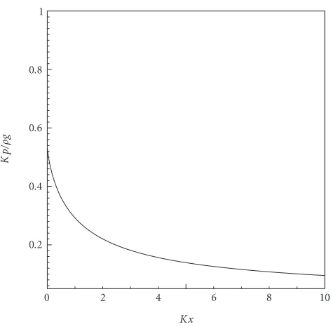
Similarly, the pressure on the dockp(x,t) (x >0) is obtained as
p(x,t)=ρg
K Re
iφ(x, 0)e−iσt=ρg
K
√ 2
π sin
π
8 +σt
J(Kx), (3.3)
where
J(s)= π/2
0 exp
−scotθ+sinθ
π
π/2
0
α
sinαsin(θ+α)dα
dθ. (3.4)
Figures 3.1and3.2depict, respectively, the free surface profileη(x, 0) againstx(x <0) and the pressure distribution p(x, 0) on the dock also against x(x >0);η, p, x being nondimensionalised asKη,K p/ρg,Kx. These curves inFigures 3.1and3.2can be iden-tified with the curves given in [2] obtained from the potential function ReχR(z) given
−10 −8 −6 −4 −2 0
Kx −1
−0.5 0 0.5 1
[image:7.468.117.354.71.299.2]Kη
Figure 3.1. Free surface profile att=0.
0 2 4 6 8 10
Kx 0.2
0.4 0.6 0.8 1
Kp
/ρ
g
[image:7.468.115.351.341.574.2]Appendices
A. Determination ofC(ξ)
In this appendix we will describe the contour integration procedure to obtain the value ofC(ξ), as given by the relation (2.22).
The relation (2.20) gives
C(ξ)=Φ+(ξ)−Φ−(ξ)= − Kξ
ξ+iK
R ξ2+K2+
1 (ξ−iK)2
−K2Φ+0(ξ)
π(ξ+iK) ∞
0
R u2+K2+
1 (u−iK)2
1 Φ+
0(u)(u−ξ)
du, ξ >0.
(A.1)
The integrals appearing in (A.1) can be evaluated by considering integrals of the form
I(ζ)=
Γ
P(τ)
Q(τ) 1
Φ0(τ)(τ−ζ)dτ, (A.2)
withΓa positively oriented closed contour consisting of a loop around the positive real axis and a circle of large radius with centre at the origin, in the complexτ-plane, andP(τ) andQ(τ) are polynomials inτ. If these polynomials are such that the contribution to the integral in (A.2) over the circle of large radius vanishes, then
I(ζ)=
Γ
P(u)
Q(u)
1 Φ+
0(u)− 1 Φ−
0(u)
1 (u−ζ)du
= −2iK
∞
0
P(u)
Q(u)
1 Φ+
0(u)(u−iK)(u−ζ)
du
(A.3)
after using the relation
Φ+ 0(ξ)=
ξ+iK ξ−iKΦ
−
0(ξ). (A.4)
Thus by usingP(τ)=1 andQ(τ)= −2iK(τ+iK), it is observed that
I1(ζ)= ∞
0
1
u2+K2Φ+
0(u)(u−ζ)
du
= − 1 2iK
Γ
dτ
(τ+iK)Φ0(τ)(τ−ζ)
= −π
K
1
ζ+iK
1 Φ0(ζ)−
1 Φ0(−iK)
.
Similarly, by choosingP(τ)=1 andQ(τ)= −2iK(τ−iK) in (A.3),
I2(ζ)= ∞
0
1 (u−iK)2Φ+
0(u)(u−ζ)
du
= − 1 2iK
Γ
dτ
(τ−iK)Φ0(τ)(τ−ζ)
= −π
K
1
ζ−iK
1 Φ0(ζ)−
1 Φ0(iK)
.
(A.6)
Using Plemelj’s formulae,
∞
0
1
u2+K2Φ+
0(u)(u−ξ)
du=1 2{I
+
1(ξ) +I1−(ξ)}
=π
K
1
ξ+iK
1 Φ0(−iK)−
ξ
(ξ−iK)Φ+0(ξ) , (A.7) ∞ 0 1 (u−iK)2Φ+
0(u)(u−ξ)
du=1 2
I+
2(ξ) +I2−(ξ)
= π
K
1
ξ−iK
1 Φ0(iK)−
ξ
(ξ−iK)Φ+ 0(ξ)
.
(A.8)
Using (A.7) and (A.8) in (A.1),C(ξ) is obtained as
C(ξ)= − K
ξ2+K2 Φ+
0(ξ) Φ0(iK)−
KR
(ξ+iK)2 Φ+
0(ξ)
Φ0(−iK), ξ >0. (A.9)
B. Proof of (2.24)
Here we will describe the details of the procedure to derive the relation (2.24). On using (2.21), we obtain
B(ξ)=(1 +R)Kξ
ξ2+K2 −
Kξ
2ξ2+K2
Φ+ 0(ξ) Φ0(iK)+R
Φ−
0(ξ) Φ0(−iK)
+K 2ξ π ∞ 0 1
u2−ξ2ξ2+K2
Φ+ 0(u) Φ0(iK)+R
Φ−
0(u) Φ0(−iK)
du.
(B.1)
The integrals in (B.1) can be evaluated by considering the integral
J(ζ)=
Γ
P(τ)
Q(τ) Φ0(τ)
whereΓis the same as in (A.2) andP(τ),Q(τ) are polynomials such that the contribution to the integral in (B.2) from the circle of large radius vanishes. We obtain
∞
0
Φ+ 0(u)
u2+K2u2−ζ2du=
π K
Φ0(ζ) 2ζ(ζ−iK)+
Φ0(−ζ) 2ζ(ζ+iK)−
Φ0(iK) (ζ2+K2)
, (B.3)
∞
0
Φ−
0(u)
u2+K2u2−ζ2du=
π K
Φ0(ζ) 2ζ(ζ+iK)+
Φ0(−ζ) 2ζ(ζ−iK)−
Φ0(−iK)
ζ2+K2
, (B.4)
whereζ=ξ+iη(ξ >0). Hence the use of Plemelj’s formulae produces ∞
0
Φ+ 0(u)
u2+K2u2−ξ2du=
π K
Φ+
0(ξ) 2ξ2+K2+
Φ0(−ξ) 2ξ(ξ+iK)−
Φ0(iK)
ξ2+K2
, (B.5)
∞
0
Φ−
0(u)
u2+K2u2−ξ2du=
π K
Φ−
0(ξ) 2ξ2+K2+
Φ0(−ξ) 2ξ(ξ−iK)−
Φ0(−iK)
ξ2+K2
. (B.6)
Using the results of (B.6) in (B.1), ultimatelyB(ξ) is obtained as
B(ξ)=K 2Φ0(−ξ)
1
(ξ+iK)Φ0(iK)+
R
(ξ−iK)Φ0(−iK)
. (B.7)
C. Evaluation ofR
C.1. Here we will prove the result (2.25). From (2.19a), we find that
lnΦ0(z)= 1
π
π/2
0 ln
z−Ktanθ z dθ (C.1) so that ln
Φ0(iK) Φ0(−iK)
= 1 π π/2 0 ln
i−tanθ i+ tanθ
dθ=iπ
4. (C.2)
Hence we obtain that
R=e−iπ/4. (C.3)
C.2. To determine the values ofcD1/π=D(say) andR, the relation (2.23) is used in the relations (2.11) and (2.13). This gives rise to the relations
1 +R=4DK2
π
∞
0
Λ+ 0(ξ)
ξ(ξ−iK)ξ2+K2dξ,
1−R=4iDK
π
∞
0
Λ+ 0(ξ)
(ξ−iK)ξ2+K2dξ.
The integrals in (C.4) can be evaluated by considering integrals of the form (A.2). Thus,
1 +R=2D
K
Λ0(iK) +Λ0(−iK),
1−R=2D
K
Λ0(−iK)−Λ0(iK)
(C.5)
so that
R=Λ0(Λ0(iK)
−iK), D=
cD1
π =
K
2 1
Λ0(−iK). (C.6)
D. Equivalence of (2.23) and (2.24)
Here we prove the following results:
Λ0(−iK) Φ0(iK) =
1
2, (D.1)
Λ+ 0(ξ) Φ0(−ξ)=
ξ
ξ+iK (D.2)
so that the expressions as given by the relations (2.23) along with (2.27) and (2.24) along with (2.25) represent the same functionB(ξ).
To show (D.1), it may be noted from (2.19a) and (2.19b) that
Φ0(iK)=exp
1 2πi
∞
0
ln((u+iK)/(u−iK))
u−iK du
,
Λ0(−iK)=exp
1 2πi
∞
0
ln((u−iK)/(u+iK))−2πi
u+iK du
.
(D.3)
Using the result
ln u−iK
u+iK
+ ln
u+iK
u−iK
=2πi, (D.4)
it is found that
Λ0(−iK) Φ0(iK) =exp
−πi1
∞
0 ln u+iK
u−iK
u
u2+K2du
=exp
−2
π
π/2
0 π
2 −θ
tanθdθ
=1
2.
(D.5)
To show (D.2), the results in (2.19b) and (D.4) are used to obtain
Λ+
0(ξ)=exp
1 2ln
ξ−iK ξ+iK
− 1
2πi
∞
0
ln((u+iK)/(u−iK))
u−ξ du
Also, from (2.19a), it is seen that
Φ0(−ξ)=exp
1 2πi
∞
0
ln((u+iK)/(u−iK))
u+ξ du
, ξ >0. (D.7)
Hence
Λ+ 0(ξ) Φ0(−ξ)=
ξ−iK
ξ+iK
1/2 exp
−πi1
∞
0 ln u+iK
u−iK
u
u2−ξ2du
. (D.8)
The integral in (D.8) can be evaluated and its value is 2πiln{(ξ2+K2)1/2/ξ}. Substituting this value in (D.8), the result in (D.2) is obtained.
Acknowledgments
We thank a learned referee for his suggestions to include the two figures in the revised paper. This work is partially supported by a research grant from CSIR, New Delhi, to B. N. Mandal, and by a postdoctoral assistance from NBHM, Mumbai, to R. Gayen.
References
[1] A. Chakrabarti,On the solution of the problem of scattering of surface-water waves by the edge of
an ice cover, Proc. R. Soc. Lond. Ser. A Math. Phys. Eng. Sci.456(2000), no. 1997, 1087– 1099.
[2] K. O. Friedrichs and H. Lewy,The dock problem, Commun. Pure Appl. Math.1(1948), 135–
148.
[3] F. D. Gakhov, Boundary Value Problems, Pergamon Press, Oxford; Addison-Wesley,
Mas-sachusetts, 1966.
[4] R. L. Holford,Short surface waves in the presence of a finite dock. I, Proc. Cambridge Philos. Soc.
60(1964), 957–983.
[5] ,Short surface waves in the presence of a finite dock. II, Proc. Cambridge Philos. Soc.60
(1964), 985–1011.
[6] N. I. Muskhelishvili,Singular Integral Equations: Boundary Problems of Function Theory and
Their Application to Mathematical Physics, P. NoordhoffN. V., Groningen, 1953.
[7] F. Ursell,The effect of a fixed vertical barrier on surface waves in deep water, Proc. Cambridge
Philos. Soc.43(1947), 374–382.
A. Chakrabarti: Department of Mathematics, Indian Institute of Science, Bangalore 560012, India E-mail address:[email protected]
B. N. Mandal: Physics and Applied Mathematics Unit, Indian Statistical Institute, 203 Barrackpore Trunk Road, Kolkata 700108, India
E-mail address:[email protected]
Rupanwita Gayen: Physics and Applied Mathematics Unit, Indian Statistical Institute, 203 Bar-rackpore Trunk Road, Kolkata 700108, India