Using Multi-objective Artificial Fish Swarm Algorithm to Solve
the Software Project Scheduling Problem
Sarah E. Almshhadany
University of Mosul –College of
Computer Sciences & Math
Software Engineering Dept.
Laheeb M. Ibrahim
University of Mosul –College of
Computer Sciences & Math
Software Engineering Dept.
ABSTRACT
In this paper, a new multi-objective artificial fish swarm algorithm was proposed based on the principles of PAES algorithm and it is used to solve SPSP. The aim of this proposal is to solve the software project scheduling problem with artificial fish swarm algorithm and to overcome some disadvantages that AFSA suffer from. The performance of the proposed algorithm was compared with another multi-objective AFSA based on the use of global information (GAFSA), in terms of speed, quality of produced solutions and complexity of algorithm operations. The results show that the proposed algorithm is faster, easier to implement, require less computations, and had obtained better nondominated solutions than the other algorithm.
General Terms
Swarm Intelligence.
Keywords
Software project scheduling problem, multi-objective optimization, artificial fish swarm algorithm.
1.
INTRODUCTION
The software project scheduling problem (SPSP) is an important process of allocating employees to tasks in software project so that completion time and cost is minimized [1][2]. It is different from the well-known resource-constrained project scheduling problem (RCPSP) in having two objectives to minimize while the RCPSP have only one (completion time), also in SPSP employees are the only resource to allocate, each of them have a group of skills and a salary, but in RCPSP there are many resources with quantitative amounts[2][3]. SPSP has a direct effect to project success, it is a project management activity where the project manager responsible for and he must use different techniques and methodologies to manage employees and tasks of the software project [1][4]. Therefore, it is essential to find optimal schedule to finish the project in the least amount of time and cost, but finding this optimal schedule is very hard since SPSP is considered a combinatorial optimization problem (COP) that has many different possible allocations between employees and tasks and each allocation has different cost and time. There are two different techniques to solve combinatorial optimization problems, the first technique is to use complete or exact methods that examine all possible allocations but this will consume time and space. Second technique is to use incomplete techniques that examine only parts of the possible allocations to find near optimal solutions in an acceptable time and effort. The incomplete techniques include heuristics and metaheuristics methods [5].The main distinguish between heuristics and metaheuristics methods that heuristics are methods designed to solve a certain problem only while metaheuristics can be adaptive to solve any optimization problem, and their search do not depend on
the properties of the problem. Some metaheuristics methods find one solution in every iteration like simulated annealing and tabu search, while others (population-based metaheuristics) find many solutions at a time and improve them in every iterations like genetic algorithm (GA), differential evolution (DE) and swarm algorithms like ant colony optimization (ACO), partial swarm optimization (PSO) and artificial fish swarm algorithm (AFSA) [6]. SPSP can be treated as a single-objective optimization problem where a weighted objective function is used to combine the two objectives of the problem together and produce one solution latter. However, this formulation does not reflect the nature of the problem in real world, so it is more realistic to treat SPSP as a multi-objective optimization problem that produce a set of nondominated solutions called pareto optimal set and it is called pareto front when it is plotted in the objective space [3]. AFSA is a swarm intelligence algorithm that simulate movement of natural fishes in the swarm and their interaction with environment and with one another through four different behaviors (Prey, swarm, follow and move). The algorithm has advantages like insensitivity to initial values, flexible search, and fault tolerance. It also have disadvantages like high computational complexity, and it is a complicated algorithm specially when it is compared with PSO that usually (with some improvements) can achieve better solutions than classical AFSA [7]. In this paper, a new multi-objective artificial fish swarm algorithm was proposed based on the principles of PAES algorithm and it is used to solve SPSP. The aim of this proposal is to solve the software project scheduling problem with artificial fish swarm algorithm and overcome some disadvantages that AFSA suffer from. The performance of the proposed algorithm was compared with another multi-objective AFSA based on the use of global information (GAFSA) [8], in terms of speed, quality of produced solutions and complexity of algorithm operations.
2.
LITRITURE REVIEW
evolutionary hyper-heuristics for SPSP. Also an adaptive selection of crossover and mutation operators is presented with new design of credit assignment method for mutation and crossover and sliding multi-armed bandit strategy for choosing crossover and mutation. All these novelties contributed in solving SPSP effectively [12]. Broderick et. al in 2016 took advantage of the properties of intelligent water drop algorithm (like inclusion of construction phase) to solve SPSP [13]. Maghsoud and Javad in 2015 used differential evolutionary algorithm with SPSP. The performance of the algorithm was better than genetic algorithm [4]. Jing X. et. al in 2015 performed an empirical study with multi-objective evolutionary algorithm using decomposition and ant colony (MOEA/D-ACO) and compared the performance of this algorithm with NSGA|| in solving SPSP. MOEA/D-ACO did not produce better solutions than NSGA|| in most complex instances but it obtain the results in less time and achieved less project duration for most instanced [14]. Leandro et. al in 2014 improved the evolutionary algorithm after performing runtime analysis to the scheduling problem. They adopted many enhancements as in fitness function, representation of crossover and mutation operators, and used normalization in employee’s dedications. The results of this approach was very successful [1]. Francisco et. al in 2014 performed a scalability analysis of eight multi-objective algorithms, they used 36 instances generated randomly that represent SPSP. The results of comparing the performance of these algorithms shows that PAES recorded best results in 34 of 36 instances. The reason of this interesting result is the operation (mutation) performed by PAES algorithm which make little modification on the individual, this keeps the search in the nondominated solutions area that is reached by the constrained of SPSP, while other algorithms perform intensive modification to individual and this makes the search leave the nondominated solutions area [3]. Broderick et. al in 2014 reviewed the metaheuristics used in solving SPSP like genetic algorithm, simulated annealing, ant colony optimization and other algorithms [5]. Broderick et. al in 2014 used a max-min ant system algorithm with hyper-cube framework to solve SPSP. The solutions were compared with other techniques and achieved good results [2]. In the other hand, many researches and improvements made on AFSA, and it was used to solve single and multi-objective optimization problems. Huabo Xiao in 2017 explained the disadvantages of using AFSA with non-linear optimizations problems like the degrade of search ability during the operation, falling in local extremum, and the accuracy of search in not high. Then he proposed new combinatorial heuristic artificial fish swarm algorithm (CHAFSA) to overcome these disadvantages and to provide new method for solving complicated non-linear optimizations problems. The results show the effectiveness of new proposal [15]. Zeqiang Z. et. al. in 2017 proposed new pareto improved artificial fish swarm algorithm (IAFSA) to solve multi-objective fuzzy disassembly line balancing problem (MFDLBP). The study show the effectiveness of the new algorithm [16]. Wei Y. et. al. in 2017 presented new method for predicting stock price trends. This method is based on the use of AFSA in training RPF neural network with dynamic adjustment of AFSA parameters (visual distance, step). The experiments results show the feasibility of the new method [17]. Ana Maria A. C. Rocha et. al. in 2016 proposed a two-swarm AFSA with an augmented lagrangian framework to solve bound constraints subproblems. The enhancements on AFSA helped in improving the search of the algorithm [6]. Yohong Z. et. al. in 2016 used AFSA to train radial basis function neural network (RBFNN). The results prove the increase of learning accuracy and the improvement of global
search [18]. Y. Y. et. al. in 2014 proposed new model for the magnetorheological elastomer (MRE) base isolator and new algorithm for parameter identification based on AFSA. The researchers discuss the high computational complexity of implementing AFSA and they suggested simplified behaviors of AFSA. They also discussed the impact of the parameters (visual distance, step) on the global search of the algorithm and they presented an approach for updating these parameters. The results show the efficiency of the new proposed algorithm [19]. Guohua F. et. al. in 2012 designed new multi-objective artificial fish swarm algorithm (MOAFSA). They used quick sort algorithm to save and maintain the nondominated solutions, and crowding distance to discard bad solutions. The performance of MOAFSA was compared with SPEA2 and NSGA-||, and the results show that MOAFSA is a good new method [20]. Mingyau J. and Kongcun Z. in 2011 presented a multi-objective AFSA based on global artificial fish swarm algorithm (GAFSA) and an external record is used to save the best nondominated solutions with quick sort algorithm and crowding distance to manage these solutions. They performed the proposed algorithm in parallel and compared its performance with classical AFSA and NSGA-||. The results indicates that the new algorithm is effective [8].
3.
PROBLEM DEFINITION
In order to create schedule for software project, all information about the project tasks and the staff must be in hand, this information can be divided to three components:
1. Tasks, which are the operations that must be performed to complete the software project. Every project has (T) tasks, each task (𝑡𝑖) has a set of skills
(𝑡𝑖𝑠𝑘𝑖𝑙𝑙𝑠) and an estimated effort (𝑡𝑖 𝑒𝑓𝑓𝑜𝑟𝑡
).
2. Task precedence graph (TPG) which explains the relationships among project tasks and their dependences. TGP is acyclic directed graph G (V, A) consist of vertex set V= {𝑡1,𝑡2, . . . , 𝑡𝑇} and arc
set (𝑡𝑖,𝑡𝑗) ֹ∈ A, denotes that task 𝑡𝑖 must finish
without interruption before task 𝑡𝑗 can start.
3. Employees are the only resource that SPSP has. Every project has (E) employees, each employee (𝑒𝑖) has a set of skills (𝑒𝑖𝑠𝑘𝑖𝑙𝑙𝑠) which is a sub set of
all different skills available in project staff members (𝑆𝐾), and has a salary (𝑒𝑖𝑠𝑎𝑙𝑎𝑟𝑦), and a maximum dedication of work (𝑒𝑖𝑚𝑎𝑥𝑑𝑒𝑑 = 1). The solution of
this problem is a matrix X= (𝑥𝑖𝑗) of size 𝐸 × 𝑇
where 𝑥𝑖𝑗 is the amount of dedication of employee
(𝑒𝑖) to task (𝑡𝑗), the summation of dedication for
each employee must not exceed their maximum dedication to avoid overwork. The amount of maximum dedication for all employees is always assumed to be 1. The objective of SPSP is to minimize both completion time and cost of the project [1] [12].
The completion time of the project is calculated as follows: 1. Calculate (𝑡𝑗𝑎ℎ𝑟) with Eq. (1) for every task which is
the amount of work that employees did to finish the task.
𝑡𝑗𝑎ℎ𝑟= 𝑥 𝑖𝑗 𝐸
𝑖=1 (1)
2. Find duration of each task in Eq. (2)
𝑡𝑗𝑑𝑢𝑟 = 𝑡𝑗
𝑒𝑓𝑓𝑜𝑟𝑡
𝑡𝑗𝑎 ℎ 𝑟
3. Find start time (𝑡𝑗𝑠𝑡𝑎𝑟𝑡) and finish time (𝑡 𝑗𝑒𝑛𝑑) of
every task.
𝑡𝑗𝑠𝑡𝑎𝑟𝑡 =
0 𝑖𝑓 ∄𝑡𝑖, 𝑡𝑖, 𝑡𝑗 ∈ 𝐴
max𝑡𝑖, 𝑡𝑖,𝑡𝑗 ∈𝐴 𝑡𝑖𝑒𝑛𝑑 𝑜𝑡ℎ𝑒𝑟𝑤𝑖𝑧𝑒
(3)
𝑡𝑗𝑒𝑛𝑑 = 𝑡
𝑗𝑠𝑡𝑎𝑟𝑡 + 𝑡𝑗𝑑𝑢𝑟 (4)
4. The total duration of the project is the duration of the last executed task in the project.
𝑝𝑑𝑢𝑟 = max𝑗 =1 𝑡𝑗𝑒𝑛𝑑 (5)
The cost of the project can be computed as follows: 1. Calculate the cost of each task.
𝑡𝑗𝑐𝑜𝑠𝑡 = 𝑒𝑖 𝑠𝑎𝑙𝑎𝑟𝑦
. 𝑥𝑖𝑗. 𝑡𝑗𝑑𝑢𝑟 𝐸
𝑖=1 (6)
2. The cost of project is the summation of cost of all tasks in the project.
𝑝𝑐𝑜𝑠𝑡 = 𝑇𝑗 =1𝑡𝑗𝑐𝑜𝑠𝑡 (7)
Scheduling in SPSP must satisfy some conditions: 1. At least one employee must handle every task.
𝑡𝑗𝑎ℎ𝑟 > 0 ∀𝑗 ∈ {1, 2, . . . , 𝑇} (8)
2. The group of employees responsible for a specific task must have all the skills required by that task.
𝑡𝑗𝑠𝑘𝑖𝑙𝑙𝑠 ⊆ 𝑖 𝑥𝑖𝑗>0 𝑒𝑖𝑠𝑘𝑖𝑙𝑙𝑠∀𝑗 ∈ {1, 2, . . , 𝑇} (9)
3. The work associated with each employee must not exceed the maximum dedication; first, the work of employees is computed.
𝑒𝑖𝑤𝑜𝑟𝑘 𝒯 = 𝑥 𝑖𝑗
{𝑗 |𝑡𝑗𝑠𝑡𝑎𝑟𝑡≤𝒯≤𝑡𝑗𝑒𝑛𝑑} (10)
If the work exceeds the maximum dedication (𝑒𝑖𝑤𝑜𝑟𝑘(𝒯) > 𝑒𝑖𝑚𝑎𝑥𝑑𝑒𝑑) at instant 𝒯 then an
overwork is detected.
𝑒𝑖𝑜𝑣𝑒𝑟 = 𝑟𝑎𝑚𝑝(𝑒𝑖𝑤𝑜𝑟𝑘(𝒯) − 𝑒𝑖𝑚𝑎𝑥𝑑𝑒𝑑) 𝑑𝒯 𝑟=𝑝𝑑𝑢𝑟
𝑟=0
(11)
𝑟𝑎𝑚𝑝 is a function defined as:
𝑟𝑎𝑚𝑝 𝑥 = 𝑥 𝑖𝑓 𝑥 > 0
0 𝑖𝑓 𝑥 ≤ 0 (12)
The overwork in the project is the summation of all employees overwork.
𝑝𝑜𝑣𝑒𝑟 = 𝐸𝑖=1𝑒𝑖𝑜𝑣𝑒𝑟 (13)
There is no overwork must occur in the project.
𝑝𝑜𝑣𝑒𝑟 = 0 (14)
This condition is considered the most difficult one to satisfy. When an overwork occurs, the repair operator must be used which divides all dedications of employees on the maximum overwork found:
𝑥𝑖𝑗` =
𝑥𝑖𝑗
𝑚𝑎𝑥𝑖,𝒯{𝑒𝑖𝑤𝑜𝑟𝑘 𝒯 +ℰ
(15)
Where (ℰ = 0.00001) is a value used to prevent inaccuracies in floating point operations. While using Eq. (15), the duration of the project will increase:
𝑝𝑑𝑢𝑟` = 𝑝𝑑𝑢𝑟+ 𝑚𝑎𝑥𝑖,𝒯{𝑒𝑖𝑤𝑜𝑟𝑘 𝒯 + ℰ} (16)
However, the project cost will be unaffected [3]:
𝑝𝑐𝑜𝑠𝑡` = 𝑝𝑐𝑜𝑠𝑡 (17)
4.
ARTIFICIAL FISF SWARM
ALGORITHM (AFSA)
Artificial fish swarm algorithm (AFSA) is a swarm intelligent stochastic population-based algorithm. It is a suitable choice when dealing with optimization problems as it has many great features like good global search, insensitive to initial values, robustness, easy to realize and can be implemented in parallel [18]. It have been effectively used to solve single and multi-objective optimization problems [8] and it was adopted in many application areas like improving neural networks, image segmentation, machine learning and many other fields [7]. Although the success of AFSA in many optimization areas but the researchers have conducted many drawbacks and difficulties when dealing with AFSA like the impact of parameter values (visual, step) on the convergence of the algorithm [17] [19]. When the values are constant, this slow the speed of convergence and help the algorithm in falling into a local optimum, and when they are random, this decrease the accuracy of the optimization. In addition, as the algorithm has four different behaviors, this makes it difficult to implement and this require a high computational complexity. Furthermore, if the size of the artificial fish is big, with the implementation of behaviors in parallel this require a storage space [19]. Therefore, after studying AFSA and SPSP, new improvements was suggested to enhance the performance of the algorithm when dealing with multi-objective problems, and to overcome these difficulties.
4.1
Description of Classical AFSA
AFSA has two main effective parameters: visual distance, which determine the vision of the artificial fish (AF) in the environment, and step that determine the movement of AF to the target. The algorithm has four different behavior (prey, swarm, follow and move) that simulate decisions of AF in water and how they seek for food and safety. In the following, we describe each behavior:
1. Prey behavior: If 𝑥𝑖 is the current state of AF, then it
choose randomly a new state 𝑥𝑗 in its visual
distance.
𝑥𝑗 = 𝑥𝑖+ 𝑣𝑖𝑠𝑢𝑎𝑙 × 𝑟𝑎𝑛𝑑() (18)
If the fitness value of the new state 𝑥𝑗 (𝑦𝑗) is better
than fitness value of old state 𝑥𝑖 (𝑦𝑖), then AF move
toward the new state.
𝑥𝑖(𝑡+1)= 𝑥𝑖(𝑡)+ 𝑥𝑗−𝑥𝑖 (𝑡)
𝑥𝑗−𝑥𝑖
(𝑡) × 𝑠𝑡𝑒𝑝 × 𝑟𝑎𝑛𝑑() (19)
If AF generated new states for a certain number of times (try-number) but the new states were not good then AF will execute move behavior.
2. Swarm behavior: If 𝑥𝑖 is the current state of AF,
then 𝑥𝑐 is the center position, 𝑛𝑓 is the number of
AF that their distance (𝑑𝑖𝑗) is less than visual (𝑑𝑖𝑗 <
visual), and 𝑛 is the total number of AF. If (𝑦𝑖 <𝑦𝑐)
and the area around the center position is not crowded, (𝑛𝑓/𝑛 < 𝛿) where 𝛿 is the crowding factor, then AF move toward the center position.
𝑥𝑖(𝑡+1)= 𝑥𝑖(𝑡)+ 𝑥𝑐−𝑥𝑖 (𝑡)
𝑥𝑐−𝑥𝑖
(𝑡) × 𝑠𝑡𝑒𝑝 × 𝑟𝑎𝑛𝑑() (20)
3. Follow behavior: If 𝑥𝑖 is the current state of AF,
fitness valve (𝑦𝑖 <𝑦𝑗), and area around him is not
crowded (𝑛𝑓/𝑛 < 𝛿) and their distance (𝑑𝑖𝑗) is less
than visual (𝑑𝑖𝑗 < visual), then AF move toward this
companion’s position.
𝑥𝑖(𝑡+1)= 𝑥𝑖(𝑡)+ 𝑥𝑗−𝑥𝑖 (𝑡)
𝑥𝑗−𝑥𝑖
(𝑡) × 𝑠𝑡𝑒𝑝 × 𝑟𝑎𝑛𝑑() (21)
4. Move behavior: it is the random movement of fishes in water. If 𝑥𝑖 is the current state of AF, then 𝑥𝑗 is a
random generated new state that AF moves toward it [21].
𝑥𝑗 = 𝑥𝑖+ 𝑣𝑖𝑠𝑢𝑎𝑙 × 𝑟𝑎𝑛𝑑() (22)
4.2
AFSA with Global information
(GAFSA)
This multi-objective algorithm uses the concept of adding the global information (best AF in the swarm) in updating every behavior along with the local information of that behavior, this increase the diversity of the population and prevent the AF from gathering in one area. The work in the algorithm is conducted in parallel as shown in this procedure:
1. Generate initial random swarm, and set parameters of the algorithm.
2. Calculate the pareto optimal solutions and sort them with quick sort algorithm, save them in the external record set.
3. With the aid of crowding distance, determine the global information.
4. Perform four behaviors on every AF and choose the behavior of best results (in the mean of pareto dominance relationship).
5. Updated AF with global information and local information. Save the found solutions in nondominated set.
6. Add the nondominated set to external record set and update it by using quick sort algorithm and crowding distance.
7. Check the stopping condition, if it is satisfied output the external record, and if it is not return to step 3 [8].
4.3
The Proposed Algorithm
The motivation of this new proposal is the excellent results reached by PAES algorithm in solving SPSP that was proved in [3]. PAES algorithm is extremely different from AFSA, it works every iteration on one individual and it uses one operator (mutation) in modifying this individual so it does not suffer from complexity like AFSA, also the simple modification was successful in finding nondominated solutions better than other algorithm. This good result is explained as follows: As SPSP has three conditions that must be satisfied by every individual, this leads the global search to the local area of the nondominated solutions. Now the algorithm should discover this area to find these solutions, so the little modification (as in PAES) is preferred here more than the intensive modification (as in other algorithms and in AFSA) that will lead the search to be out of the nondominated solution area. This prove that the complexity and parallelism of AFSA is not necessary. Diversity of nondominated solutions is an important issue, the algorithm should search the entire area of the pareto optimal solutions not only a part of it. PAES
chooses the best individual to be the individual of the next iteration while GAFSA uses global information to maintain diversity but this increase the complexity of the algorithm. Another important criterion, which is the perform of repair factor. When the algorithm makes little modification to the individual this means that it does not need to perform repair operator, but when the modification is intensive, the algorithm must handle the burned of performing repair operator that increase the computation and execution time of the algorithm, also the duration of the project.
The aim of the new proposal is to satisfy these goals:
1. The new algorithm must be faster than GAFSA, which is an important criterion when developing a scheduling tool for the project manager based on SPSP. This is measured by the execution time. 2. It should be less difficult to implement than
GAFSA; this is measured by the percentage of performing repair operator.
3. The quality of solutions founded by the new algorithm should be higher than the solutions produced by GAFSA. The hypervolume indicator (HV) measures this quality.
HV is one of the best indicators that used to measure the quality of solutions and the dominated region obtained by the multi-objective optimization algorithms. It is a sensitive metric to convergence and diversity of the nondominated sets, the more higher values of HV indicator the better it is [3]. In order to perform little modification on AF, the proposed algorithm apply one new behavior that works on one random pixel of AF. This behavior add the value of step to the random pixel and as the step should be inside the vision of AF, this summation is divided on the value of visual that is multiplied with a random value between (0,1), which is (the random value) the important element of the stochastic search, the work is summarized by this equation:
𝐴𝐹 𝑖,𝑗 ′ =
𝐴𝐹(𝑖,𝑗 )+𝑠𝑡𝑒𝑝
𝑣𝑖𝑠𝑢𝑎𝑙 +𝑟𝑎𝑛𝑑 () (23)
This helps the algorithm to keep the local search in the nondominated area reached throw the constrained of SPSP. The use of this new behavior either give new assignment (if the random pixel was equal to zero) or increase or decrease the assigned pixel but it does not cancel any assignment given in the random population. Therefore, another operation is performed (similar to mutation operator) that give the value of zero to random pixel from the same AF, as in the following equation:
𝐴𝐹 𝑥,𝑦 ′ = 0 (24)
The new behavior decrease the complexity of the algorithm, the execution time, and the times where performing the repair operator is needed. The nondominated solutions is kept in the external record set ant it managed by the quick sort algorithm. The diversity of the AF in the swarm and the diversity of the founded solutions is maintained by choosing the best AFs from the old and the new swarm to be the swarm of the next iteration. These best AFs is determined by calculating the crowding distance (browed from NSGA-||) and choosing AFs with highest values. This measure is also used to discard the bad nondominated solutions when they exceed the limit of the external record set. The procedure of the new algorithm is described as follows:
2. Calculate the pareto optimal solutions and sort them with quick sort algorithm, save them in the external record set.
3. Perform the new behavior and the new operator on every AF, and save the found solutions in nondominated set.
4. Add the nondominated set to external record set and update it by using quick sort algorithm and crowding distance.
5. Choose best AFs (by the value of crowding distance) to be the swarm of next iteration.
6. Check the stopping condition, if it is satisfied output the external record, and if it is not return to step 3.
5.
THE EXPEREMENT
The experiment was conducted using matlab R2017a, and in windows 10 Pro, CPU 2.50GHz-2.70GHz and 4 GB RAM. The parameters of both algorithms is summarized in table 1:
Table1. The parameters of the algorithms
Parameter Proposed
algorithm GAFSA
Behaviors New behavior, New operator
Prey, swarm, follow and move
Visual distance 1.5 1.5
Step 0.01 0.01
AFs number 20 20
Nondominated
record size 20 20
External
Record size 100 100
Iteration
number 1000 1000
Run number 10 10
The data used in this study is the same 36 instances used in [3], each represent a different software project. The number of tasks ranges from 16 to 512 while the number of employees ranges from 8 to 256. Each task and employee has 6 to 7 different skills from the total 10 skills. The instances was represented as I T-E where T is the number of tasks and E is the number of employees. In order to study the effect of the new behavior and the real result of the little modification that was performed on every AF, and also to design a fast multi-objective AFSA, these decision was made:
1. The mechanism of determining the swarm of every iteration was performed in GAFSA as well, in order to leave the performing of the behaviors as the main difference between the two algorithms and to be certain that the difference in performance is caused by implementation of the behaviors and not because this mechanism adopted by the new algorithm. 2. Calculating the distance between two AFs when
performing swarm and follow behavior is very difficult and consume time specially that the smallest size of AF is (8*16). Therefor 𝑥𝑐 (in swarm
behavior) is determined as the AF with the middle value of crowding distance, and 𝑥𝑗 (in follow
behavior) is any AF in the swarm which has bigger crowding distance value than the current AF. If the current AF is the global information, (the best AF
that has the highest crowding distance value) then 𝑥𝑗
is the second best AF in the swarm.
6.
RESULTS
[image:5.595.314.543.186.774.2]1. Execution time: after using both algorithms in solving SPSP, the difference in the execution time was clear. Table 2 shows the average execution time (in seconds) of the 10 runs of each algorithm and for all the instances. The colored values is the better values.
Table 3. The average execution time
Instances
Execution time (seconds) of the proposed algorithm
Execution time (seconds) of the GAFSA
I 16-8 1.743563 6.133301
I 16-16 1.791684 6.812029
I 16-32 2.427282 10.14766
I 16-64 3.179088 13.36475
I 16-128 5.211195 8.805565
I 16-256 9.678788 32.38399
I 32-8 2.616040 10.14821
I 32-16 2.963362 11.66013
I 32-32 4.196267 17.51498
I 32-64 5.698720 24.13339
I 32-128 10.69465 43.89677
I 32-256 19.68083 70.60811
I 64-8 4.293080 18.47061
I 64-16 5.041200 20.56367
I 64-32 7.976621 36.10802
I 64-64 11.77743 38.48498
I 64-128 21.33726 61.43580
I 64-256 40.78341 175.7465
I 128-8 8.479430 37.40775
I 128-16 7.150500 26.01857
I 128-32 11.53540 40.68323
I 128-64 22.23405 81.68272
I 128-128 43.80979 173.2935
I 128-256 88.98694 306.8826
I 256-8 15.91626 67.59568
I 256-16 22.94362 100.1931
I 256-32 32.52907 136.6287
I 256-64 56.92229 209.0573
I 256-128 97.27130 380.6036
I 256-256 194.1337 752.2993
I 512-16 65.93876 313.1289
I 512-32 71.86159 315.4627
I 512-64 127.5580 543.7675
I 512-128 205.7918 751.6812
I 512-256 413.6490 1503.578
[image:6.595.53.283.236.757.2]2. Repair operator: as the modification on the AF is less in the proposed algorithm than in GAFSA, it is expected to be performed less in the proposed algorithm. Table 3 shows the average percentage of performing the repair operator in both algorithm.
Table 4. The percentage of performing repair operator
Instances
Repair operator (percentage) of the proposed algorithm
Repair operator (percentage) of the GAFSA
I 16-8 11.63750 94.5965
I 16-16 6.358 95.9425
I 16-32 3.7995 95.7705
I 16-64 2.3145 98.1345
I 16-128 1.558 97.81
I 16-256 1.176 96.8275
I 32-8 13.5045 99.7755
I 32-16 6.7635 96.527
I 32-32 3.873 96.328
I 32-64 2.33 97.8885
I 32-128 1.516 98.2825
I 32-256 1.1725 97.8605
I 64-8 13.1925 99.848
I 64-16 6.8875 96.5285
I 64-32 3.8965 99.181
I 64-64 2.402 96.479
I 64-128 1.5625 97.8575
I 64-256 1.113 97.587
I 128-8 14.258 99.871
I 128-16 7.1435 99.832
I 128-32 3.9715 99.9375
I 128-64 2.3835 99.936
I 128-128 1.581 99.923
I 128-256 1.133 97.692
I 256-8 14.3575 96.6615
I 256-16 7.158 96.8295
I 256-32 3.9965 99.958
I 256-64 2.354 96.458
I 256-128 1.5815 99.985
I 256-256 1.197 96.7775
I 512-8 15.442 96.4925
I 512-16 7.396 96.4495
I 512-32 4.072 99.977
I 512-64 2.414 99.982
I 512-128 1.618 96.5215
I 512-256 1.171 96.4395
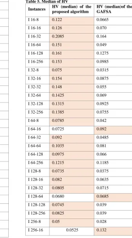
[image:6.595.263.536.271.760.2]3. Median of HV: this indicator explain the diversity and the quality of the founded nondominated solutions. Table 4 shows the median of HV for both algorithms.
Table 5. Median of HV
Instances HV (median) of the proposed algorithm
HV (median)of the GAFSA
I 16-8 0.122 0.0665
I 16-16 0.126 0.070
I 16-32 0.2085 0.164
I 16-64 0.151 0.049
I 16-128 0.161 0.1275
I 16-256 0.153 0.0985
I 32-8 0.075 0.0315
I 32-16 0.154 0.0875
I 32-32 0.148 0.055
I 32-64 0.1425 0.069
I 32-128 0.1315 0.0925
I 32-256 0.1385 0.0755
I 64-8 0.0785 0.042
I 64-16 0.0725 0.092
I 64-32 0.092 0.0485
I 64-64 0.1035 0.081
I 64-128 0.0975 0.066
I 64-256 0.1215 0.1185
I 128-8 0.0735 0.0375
I 128-16 0.082 0.0635
I 128-32 0.0805 0.0715
I 128-64 0.0680 0.0685
I 128-128 0.0745 0.039
I 128-256 0.0825 0.039
I 256-8 0.05 0.028
I 256-32 0.0545 0.027
I 256-64 0.049 0.035
I 256-128 0.06 0.045
I 256-256 0.054 0.024
I 512-8 0.0145 0.0135
I 512-16 0.0305 0.0485
I 512-32 0.030 0.0295
I 512-64 0.027 0.048
I 512-128 0.0305 0.057
I 512-256 0.029 0.0455
7.
DISSCUTION
After observing table 2, it is easy to distinguish the huge difference of time between the two algorithms. The main reason is certainly the limited and the intensive operations that was performed on the AF. The proposed algorithm took advantage of the properties of SPSP (as a constrained multi-objective optimization problem) and it did not apply but the necessary steps to discover the nondominated solution area, and it is considered more suitable for software tools and applications than GAFSA. Table 3 provide another reason for the difference in execution time. The percentage of performing the repair operator is extremely big when GAFSA is implemented. Another observation that in the proposed algorithm, the percentage of applying the repair operator decreases with the increment of SPSP instances (due to the big size of AF) that reduces the work on the algorithm when the data and the size of AF are big. However, this percentage remain high with all the instances when using GAFSA, so the amount of work and the computational complexity is always high for this algorithm. Table 4 shows that the proposed algorithm was able to find better and more diverse nondominated solutions in 26 instances than those where founded by GAFSA. This prove that the new proposal was successful and the little modification was enough to find good results than the unnecessary implementation of the four behaviors in GAFSA. This also eliminates the impact of visual and step as the goal of the local search is only to discover the area of nondominated solutions and not the entire global search area.
8.
CONCLUTIONS AND FUTUER
WORK
The results of the experiment show that the proposed algorithm is faster, easier to implement, and require less computation than the other algorithm. It achieved successfully all the three predefined goals. The results of this experiment can be used to compare the performance of AFSA with other swarm intelligence algorithms. The performance of the algorithm can be further studded by determining a percentage of modification rather than applying it on one pixel of AF, this might increase the diversity of solutions. In addition, the initial values of visual and step can be further investigated. Furthermore, the algorithm can be used to solve other multi-objective optimization problems similar to SPSP.
9.
REFERENCES
[1] Leondro L M., Dirk S., Xin Y. 2014. Improved evolutionary algorithm design for the project scheduling
problem based on runtime analysis. IEEE. Vol.40-No.1, pp. 83-102.
[2] Broderick C., Ricardo S., Franklin J., Eric M., Fernando P. 2014. A max-min ant system algorithm to solve the software project scheduling problem. Expert System with Applications. Vol.41-No.15, pp. 6634-6645.
[3] Francisco L., David L G., Francisco C., Miguel A V. 2014. The software project scheduling problem: A scalability analysis of multi-objective metaheuristics. Applied Soft Computing. Vol.15, pp. 136-148.
[4] Maghsoud A., Javad Pashaei B. 2015. New approach for solving software project scheduling problem using differential evolutionary algorithm. International Journal in Foundation of Computer Science and Technology (IJFCST). Vol.5-No.1.
[5] Broderick C., Ricardo S., Franklin J., Sanjay M., Fernando P. 2014. The use of metaheuristics to software project scheduling problem. In International Conference on Computational Science and It's Application. Springer. pp. 215-226.
[6] Ana Maria AC R., M. Fernanda P C., Edite M.G.P. F. 2016. A shifted hyperbolic augmented lagrangian-based artificial fish two-swarm algorithm with guarantee convergence for constrained global optimization. Engineering Optimization. Vol.48-No.12. pp. 2114-2140.
[7] Reza A. 2014. Empirecal study of artificial fish swarm algorithm. arXiv preprint aeXiv:1405.4138.
[8] Mingyan J., Kongcun Z. 2011. Multi-objective optimization by artificial fish swarm algorithm. In Computer Science and Automation Engineering (CSAE) 2011 IEEE International Conference. IEEE. Vol.3. pp. 506-511.
[9] Valdi R., M Anwar M. 2017. Comparative analysis of ant colony extended and mix-min ant system in software project scheduling problem. In Big Data and Information Security (IWBIS), 2017 International Workshop on. IEEE. pp. 85-91.
[10] Natash N. 2017. Model-based dynamic software project scheduling. In Proceedings of 2017 11th Joint Meeting on Foundations of Software Engineering. ACM. pp. 1042-1045.
[11] Broderick C., Ricardo S., Franklin J., Carlos V., Fernando P. 2016. Firefly Algorithm to Solve a Project Scheduling Problem. In Artificial Intelligence Perspective in Intelligent Systems. Springer. pp. 449-458.
[12] Xiuli W., Pietro C., Leandro M., Gabriela O., Xin Y. 2016. An evolutionary hyper-heuristic for the software project scheduling Problem. In International Conference on Parallel Problem Solving from Nature. Springer. pp.
[13] Broderick C., Ricardo S., Gino A., Eduardo O. 2016. Intelligent water drop algorithm (IWD) to solve software project scheduling problem. In Information Systems and Technologies (CISTI), 2016 11th Iberian Conference on. IEEE. pp. 1-4.
Annual Conference on Genetic and Evolutionary Computation. ACM. pp. 759-766.
[15] Huabo X. 2017. Application of combinatorial Heuristic Artificial Fish Swarm Algorithm in Non-linear Optimization Problems. Boletin Tecnico. Vol.55-No.5. pp. 174-180.
[16] Zeqiang Z., Kaipu W., Lixia Z., and Yi W. 2017. A Pareto improved artificial fish swarm algorithm for solving a multi-objective fuzzy disassembly line balancing problem. Expert Systems with Applications. Vol.86. pp. 165-176.
[17] Wei Y., Gan X., Lei L. 2017. Stock Price Trend Prediction Based on RBF Neural Network and Artificial Fish Swarm Algorithm.
[18] Yuhong Z., Jiguang D., Limin S. 2016. Application of Artificial Fish Swarm Algorithm in Radial Basis Function Neural Network. TELKOMNIKA
(Telecommunication Computing Electronics and Control). Vol.14-No.2. pp. 699-706.
[19] Y Y., Y L., J L. 2014. A new hysteretic model for magnetorheological elastomer base isolator and parameter identification based on modified artificial fish swarm algorithm. In ISARC. Proceedings of the International Symposium on Automation and Robotics in Construction. Vilnius Gediminas Technical University, Department of Construction Economics and Property. Vol.31. pp. 1.
[20] Guohua F., Wei G., Xianfeng H., Xinyi S., Fei Y., Qian L., Ke Y. 2012. A new multi-objective optimization algorithm: MOAFSA and its application. Przegląd Elektrotechniczny. Vol.88-No.9b. pp. 172-176.