Using Graph Partitioning for Scalable Distributed Quantum
Molecular Dynamics
Hristo N. Djidjev∗ Georg Hahn† Susan M. Mniszewski∗ Christian F.A. Negre∗ Anders M.N. Niklasson∗ Vivek B. Sardeshmukh‡
Abstract
The simulation of the physical movement of multi-body systems at an atomistic level, with forces calculated from a quantum mechanical description of the electrons, motivates a graph partitioning problem studied in this article. Several advanced algorithms relying on evaluations of matrix polynomials have been published in the literature for such simulations. We aim to use a special type of graph partitioning in order to efficiently parallelize these computations. For this, we create a graph representing the zero-nonzero structure of a thresholded density matrix, and partition that graph into several components. Each separate submatrix (corresponding to each subgraph) is then substituted into the matrix polynomial, and the result for the full matrix polynomial is reassembled at the end from the individual polynomials. This paper starts by introducing a rigorous definition as well as a mathematical justification of this partitioning problem. We assess the performance of several methods to compute graph partitions with respect to both the quality of the partitioning and their runtime.
1
Introduction
The physical movements of multi-body systems on an atomistic level is at the core of molecular dynamics (MD) simulations. Those dynamics take place at the femtosecond (10−15 second) time
scale and they are incorporated in a larger simulation which typically is of the order of pico- to nanoseconds (10−12 to 10−9 second). A simple way to conduct MD simulations is to derive all forces from the potential energy surface for all the interacting particles, and to compute molecular trajectories for the multi-particle system by solving Newton’s equations numerically. In quantum-based molecular dynamics (QMD) simulations, the electronic structure is quantum-based on an underlying quantum mechanical description, from which interatomic forces are calculated.
Several QMD methods are published in the literature for a variety of materials systems. So-called first principle methods are capable of simulating a few hundred atoms over a picosecond range. Important approaches of this type include Hartree-Fock or density functional theory. Semiempirical methods such as self-consistent tight-binding techniques increase the applicability to systems of several thousand atoms. In contrast to regular first principle methods, approximate methods are often two to three orders of magnitude faster while still capturing the quantum me-chanical behavior (for example, charge transfer, bond formation, excitations, and quantum size effects) of the system.
∗
Los Alamos National Laboratory, Los Alamos, NM 87544, USA
†
Lancaster University, Bailrigg, Lancaster LA1 4YW, U.K.
‡
University of Iowa, Computer Science Department, Iowa City, IA 52242, USA
One of the most efficient and widely used methods is density functional based self-consistent tight-binding theory (Elstner et al., 1998; Finnis et al., 1998; Frauenheim et al., 2000). In this approach, the main computational effort stems from the diagonalization of a matrix, the so-called
Hamiltonian matrix, which encodes the electronic energy of the system. The Hamiltonian matrix is needed in order to construct thedensity matrix describing the electronic structure of the system. Before evaluating the forces at each time step of a QMD simulation, the self-consistent construction of the density marix is carried out. Computing the density matrix requires matrix diagonalization with a computational cost of O(N3), where N is the dimension of the Hamiltonian. This makes
diagonalization only viable for small system sizes. For this reason, the last two decades have seen the development of a number of linear runtime (i.e., O(N)) algorithms.
One such linear runtime approach is based on a recursive polynomial expansion of the density matrix (Niklasson, 2002). A linear scaling with the system size for non-metallic systems is achieved by the sparse-matrix second-order spectral projection (SM-SP2) algorithm. On dense or sparse matrices, SM-SP2 competes with or outperforms regular diagonalization schemes with respect to both speed and accuracy (Mniszewski et al., 2015). SM-SP2 uses the expression
D= lim
i→∞fi[fi−1[. . . f0[X0]. . .]] (1) to compute the density matrix D from the Hamiltonian H, where fi(Xi) is a quadratic function
(either X2
i or 2Xi−Xi2, depending onT r(Xi) or T r(Xi+1)) and the initial matrix X0 is a linearly
modified version of H. Usually, 20−30 iterations suffice to obtain a close approximation of D. Additionally, thresholding is applied to further reduce the computational complexity, where small nonzero elements of the matrix (typically between 10−5 to 10−7) are set to zero.
The cost of computing a matrix polynomialP (which is mainly due to the squaring of a matrix) dominates the computational cost of the SM-SP2 algorithm. Since we are interested in performing a large number of time steps (of the order of 104−106) in a typical QMD simulation, we need to
parallelize the evaluation of the matrix polynomials in order to keep the wall-clock time low. How-ever, the significant communication overhead for every iteration causes SM-SP2 to not parallelize well. Linear scaling complexity has been achieved with thresholded blocked sparse matrix algebra (Bock and Challacombe, 2013; Borstnik et al., 2014; Mniszewski et al., 2015; VandeVondele et al., 2012). In our paper, we present an alternative formulation that reduces communication overhead via graph partitioning and enables scalable parallelism. Our basic approach was introduced in Niklasson et al. (2016), but with the main focus being on the physics aspects.
This paper addresses the aforementioned parallel version of SP2 together with an inbuilt par-titioning scheme applied to the graph representation of the density matrix, denoted as G-SP2 in the remainder of the article. In particular, the computational aspects of evaluating the matrix polynomial in G-SP2 are investigated. We represent the Hamiltonian (or density) matrix as a graph where atomic orbitals are given as vertices and non-zero interactions become edges, and then partition that graph into parts (or partitions) with the aim to minimize a suitable cost function. The submatrices of the Hamiltonian or density matrix correspond to the divisions of the molecule, and are derived from the graph partitions. We show that applying the full matrix polynomial to the unpartitioned matrix is equivalent to combining the results obtained by applying the matrix polynomials to each submatrix independently.
edge cut minimization. In our article, we will experimentally study several algorithms for the aforementioned graph partitioning problem, which we formally introduce first.
We rigorously prove that applying the matrix polynomial to the entire Hamiltonian is equivalent to applying it to the partitioned Hamiltonian matrix and re-assembling the partial solutions, thus justifying our approach to parallelize the computational workload via graph partitioning. Although demonstrated numerically (Niklasson et al., 2016), no such proof exists in the literature to the best of our knowledge.
Regular graph partitioning, defined as the task of separating the vertices of a graph into roughly equal sets that minimize the edge cut between them, has been studied extensively from theoretical and applied aspects. Graph separators form the basis of many divide-and-conquer algorithms for problems such as VLSI design, shortest paths finding, solving sparse systems of linear equations, and approximations of NP-hard problems in theoretical computer science (Lipton and Tarjan, 1979; Aleksandrov and Djidjev, 1996; Miller, 1997; Wulff-Nilsen, 2011). Graph separator algorithms produce balanced partitions for graphs from a given class. The separator is a set of vertices or edges whose removal divides the graph, which usually has size bounded by a small function of the graph parameters. Although theoretical results on graph separators are usually asymptotically optimal, those are still too impractical for applications due to the fact that their leading constants are often too large. A class of graph partitioning tools has been devised which is based on heuristics such as Kernighan-Lin (Kernighan and Lin, 1970) and multilevel optimization Hendrickson and Leland (1995). Available software using those techniques include Chaco (Hendrickson and Leland, 1995), METIS (Karypis and Kumar, 1999), Jostle (Walshaw and Cross, 2000), and KaHIP (Sanders and Schulz, 2011). The advantage of such tools consists in the fact that the input graph is not required to belong to a certain class of graphs (such as planar graphs or graphs of bounded genus). Moreover, those tools usually return partitions of good quality, yet without provable quality bounds. Existing algorithms optimize the size of the cutset as objective function, whereas our work focuses on a new flavor of the graph partitioning problem with overlapping partitions.
Thresholding the matrix elements of the Hamiltonian is essential in order to arrive at a fast way to calculate the density matrix: without thresholding, the resulting matrix would quickly become dense due to fill-in. The accuracy of the collected density matrix will depend on the chosen graph partitioning, though in general the effect is small and the error is controlled mainly by the numerical threshold (Niklasson et al., 2016).
Our approach allows us to avoid communication between processors after each iteration of (1) until the entire polynomial is evaluated. To this end, each processor independently evaluates its assigned polynomial after partitioning and distributing the inital matrix, and the final output is assembled from the computed submatrices. In this article, different algorithmic approaches for computing graph partitions are assessed with respect to the aforementioned objective function and their computational effort. Importantly, we analyze the tradeoff between the additional compu-tational costs for computing graph partitions before running the SP2 algorithm in parallel, and carrying out regular molecular dynamics. We also investigate the optimal number of partitions as a function of the graph size.
The structure of this paper is as follows. Section 2 introduces the mathematical foundations for partitioning the evaluation of matrix polynomials, states our algorithm including a proof of correctness, and defines the graph partitioning problem we consider. Algorithms for constructing such partitions and their implementations are discussed in Section 3. Experimental results for several physical test systems are given in Section 4. Section 5 discusses our results. Proofs for Section 2 can be found in Appendix A, and Appendix B presents further experimental results.
is an extension of the work of Djidjev et al. (2016), and includes proofs of all theoretical results of Section 2 in Appendix A, pseudo-code of our simulated annealing approach in Section 3.2, a visualization of the relationship between the graph structure of a molecule and its partitioned graph representation in Section 4.3, and more detailed performance data used for all experiments in Appendix B.
2
Evaluating Matrix Polynomials on Partitions
We define a thresholded matrix polynomial, justify its parallelized evaluation, present an algorithm to evaluate a matrix polynomial in a parallelized fashion, and conclude by defining the cost function for an implied graph partitioning problem.
We encode the zero-nonzero structure of a symmetric matrixX={xij}as a graphG(X), called
thesparsity graph ofX. G(X) contains a vertex for each row (or column) inX, andG(X) contains an edge between verticesi and j if and only if xij 6= 0. We now generalize the matrix polynomial
defined in (1) for any symmetricn×nmatrixA. Denote the superposition of operators of the type
P =P1◦T1◦. . .◦Ps◦Ts (2)
as a thresholded matrix polynomial of degree m = 2s, where Ti is a thresholding operation and
Pi is a polynomial of degree 2. For any graph I, we formally define Ti as the graph operator
(with associated edge setE(Ti)) such thatTi(I) is a graph with a vertex set V(I) and an edge set
E(I)\Ti.
The application of a superpositioned operator P of the type (2) to a matrix A of appropriate dimension is denoted as P(A). Analogously to (2),P is composed of polynomials Pi and
thresh-olding operations Ti. For our SM-SP2 application, the Hamiltonian is A and the density matrix is
P(A).
For any matrix A, we define all matrices B which have the same zero-nonzero structure as A (that is, G(A) =G(B)) to be in the structure classM(A).
Let G =G(A) for a matrix A and let P be a thresholded matrix polynomial. With P(G) we denote the minimal graph with the same vertices as G such that if P(B)|vw 6= 0 for any matrix
B ∈ M(A) and anyv, w, then there is an edge (v, w)∈E(P(G)). We interpretP(G) as the worst-case zero-nonzero structure of P(A) which excludes cancellations resulting from the addition of opposite-sign numbers, thus resulting in coincidental zeros. All diagonal elements ofAare assumed to be non-zero, andE(Ti) is assumed to not contain a loop edge.
Assume we are given a collection of partitions Π ={Π1, . . . ,Πq}. Each partition Πi=Ui∪Wi
is a union of acore vertex setUi and ahalo vertex setWi. Given the two following conditions hold
true, we call Π a CH-partition (or core-halo partition):
1. S
iUi=V(G), Ui∩Uj =∅ for alli6=j;
2. neighbors of vertices in Ui that are themselves not inUi are contained inWi.
LetHUi be the subgraph ofH=P(G) induced by all neighbors ofUi inH. We combine all rows
and columns of A that correspond to vertices of V(HUi) in a submatrix AUi of A. The following
lemma shows thatP(A) can be computed on submatrices of the Hamiltonian.
Lemma 1. For any v ∈Ui and any neighbor w of v in P(G), the element of P(A) corresponding
Lemma 1 justifies the parallelized evaluation of a matrix polynomial.
Let us apply the aforementioned results to a Hamiltonian matrix A in a QMD simulation. In this case, we can assume that the sparsity structure of the density matrix D from the previous QMD simulation step is being passed on toP(A). We can thus approximateH=P(G) withG(D) (the graphHis unknown untilP(A) is computed). The halos can also be taken fromH in practice.
We propose the following algorithm for computing P(A) from H=G(D):
1. Divide V(G) into q disjoint sets {U1, . . . , Uq} and define a CH-partition Π = {Π1, . . . ,Πq},
where Πi has core Ui and halo N(Ui, H)\Ui;
2. Construct submatrices AUi for all i= 1, . . . , q;
3. Compute P(AUi) for all iindependently using dense matrix algebra;
4. Define P(A) as a matrix whose i-th row has nonzero elements equal to the corresponding elements of the j-th row ofP(AUk), where Uk is the set containing vertex iand j is the row
inAUk corresponding to thei-th row in A.
This algorithm computes P(A) as demonstrated in Lemma 1.
The computational bottleneck of the algorithm for P(A) is caused by the dense matrix-matrix multiplication required to compute P(AUi) for all iin step (iii).
To be precise, according to (2), computing P(AUi) takess(ci+hi)
3 operations, wherec
i andhi
are the size of the core and the halo of Πi and s is the number of superpositioned operators (see
(2)). In this calculation, the computational effort for thresholding some matrix elements is excluded, since this effort is quadratic in the worst case and linear in ci+hi in average cases. We observe
that a CH-partition which minimizes the effort to compute P(A) also minimizes Pq
i=1(ci +hi)3
due to the fact that sis independent of Π.
This observation motivates our CH-partitioning problem, defined as follows: For an undirected graphG and an integerq ≥2, split Gintoq parts Π1, . . . ,Πq such that
q X
i=1
(ci+hi)3 (3)
is minimized, where Πi has a core Ui of size ci and a haloN(Ui, G)\Ui of sizehi.
As an example, the optimal CH-partitioning for a star graph ofnvertices has a single non-empty part containing all vertices: this part is composed of the central vertex, whose halo contains all other vertices. In contrast, a standard (edge cut) partitioning will havenparts, thus demonstrating that a CH-partitioning minimizing (3) can be quite different from a standard balanced partitioning.
3
Algorithms for Graph Partitioning Considered in our Study
In this section we investigate the ability of existing graph partitioning packages, as well as our own heuristic algorithm, for computing CH-partitions that minimize the objective function (3). Those algorithms are: METIS and hMETIS due to their widespread use, and KaHIP based on its convincing performance at the 10th DIMACS Implementation Challenge Bader et al. (2013).
3.1 Edge Cut Graph Partitioning
We observe that we obtain |V(G)|+P
ihi when leaving out the cubes in the objective function
Regular graph partitions and CH-partitions are related. Suppose we are given a regular partition P. For any part in P, we can define a core corresponding to that part, and a halo consisting of all adjacent vertices of the core vertices (excluding the core vertices themselves). We define the CH-partition Π to consist of precisely those parts and halos for any element of P. It must then be true that eitherv orwis a halo vertex for any cut edge (v, w) ofP. Conversely, there exists a core vertex wsuch that (v, w) is a cut edge for any halo vertexv belonging to some part in Π.
This shows that the cut edges ofP and the set of halo nodes in Π are related but not equal. We observe that another measure, the total communication volume, exactly corresponds to the sum of halo nodes. Certain tools likeMETIS allow us to optimize with respect to the total communication volume. By ignoring the cubes in (3), we aim to study how well CH-partitions can be produced by regular graph partitioning tools. Additionally, we improve the solutions obtained by standard graph partitioning tools with our own heuristic in Section 3.2. The three following algorithms will be used:
3.1.1 METIS
METIS (Karypis and Kumar, 1999) uses a three-phase multilevel approach to perform graph par-titioning:
1. Starting from the original graphG=G0,METIS generates a graph sequenceG0, G1, . . . , Gn
to coarsen the input graph. The coarsening ends with a suitably small graph Gn (typically
less than 100 vertices).
2. An algorithm of choice is used to partition Gn.
3. Using the sequence Gn−1, . . . , G1, the partitions are projected back fromGn toG0.
Additionally, METIS employs a refinement algorithm such as the one of Fiduccia-Mattheyses (Fiduccia and Mattheyses, 1982) to improve the partitioning after each projection. This is nec-essary since the finer the partition, the more degrees of freedom it has during the uncoarsening phase. Several tuning parameters can be set in METIS, including the size of Gn, the coarsening
algorithm, and the algorithm used for partitioningGn.
3.1.2 KaHIP
Several multilevel graph partitioning algorithms are combined inKaHIPSanders and Schulz (2013).
KaHIP works similarly toMETIS. A given input graph is first contracted, partitions are computed on the highest contraction level, and the partitions obtained in this way are projected back to coarser levels, where refinement algorithms are used to enhance the solutions. KaHIPoffers max-flow/min-cut (Sanders and Schulz, 2011; Ford Jr. and Fulkerson, 1956), Fiduccia-Mattheyses (Fiduccia and Mattheyses, 1982) or F-cycles (Sanders and Schulz, 2011) for local improvement of the solution.
3.1.3 Hypergraph partitioning
A hypergraph formulation is an alternative approach to the classical interpretation of the den-sity matrix as an adjacency matrix (where each nonzero interaction in the denden-sity matrix is an undirected and unweighted edge).
We use hMETIS of Karypis and Kumar (2000) in order to compute hypergraph partitionings.
hMETIS is the hypergraph analog ofMETIS.
3.2 Refinement with Simulated Annealing
The objective function (3) we aim to minimize differs from the size of the edge or hyperedge cut minimized by standard graph and hypergraph partitioning algorithms. With the help the algorithm derived in this section we explicitly minimize (3).
A standard tool in optimization is the probabilistic algorithm of (Kirkpatrick et al., 1983), called simulated annealing (SA). SA iteratively proposes random modifications to an existing solution in order to improve it, and thus optimizes without gradients. If a proposed modification (or move) does not immediately lower the objective function, it might still be accepted with a certain acceptance probability. The acceptance probability is proportional to the magnitude of the (unfavorable) increase in the objective function, and antiproportional to the runtime. The latter makes it more likely for SA to accept unfavorable moves in the exploration phase at the start of each run, and it is implemented using a strictly decreasing temperature function. Modifications to the existing solution which further minimize the objective function are always accepted.
A fixed number of iterations, a vanishingly small temperature, or the lack of further improve-ments in the solution over a certain number of iterations can be employed as stopping criteria for SA.
We test the following proposal functions that return modifications to existing solutions, where a partition P is simply a set of nodes:
1. Select a random partitionP, select one of its halo nodesvat random and movevinto partition P.
2. Select a random partitionP, select one of its nodesv at random and movev intoP.
3. Like (2.) but select a random halo node v of partitionP.
4. Select the partitionP with most halo nodes and (a) move a random nodev intoP, (b) make a random halo node ofP a core node, or (c) move any node of P to another partition.
5. Like (4.) using the partition P with the largest sum of core and halo nodes.
Many more sensible proposal functions could be devised. However, in our experiments we observed that the above proposals result in a similar behavior of SA, with the best tradeoff between speed and performance being achieved by scheme (3.).
Algorithm 1 states the SA implementation we use in our experiments. Any regular (edge cut) partitioning (e.g., obtained withMETIS), and even a random partitioning, serves as input Π (the set of partitions) to Algorithm 1. The SA algorithm runs over a fixed number ofN iterations. In each iteration, we randomly select a partitionπ ∈Π as well as a random edge joining a core vertex v with a halo vertex w in π. Afterwards, π is updated withw being a core vertex. After storing the new partitioning in a set Π0, both Π and Π0 are assessed. For this we compute the change ∆ in the objective function (3) between Π0 and Π, which is used to update the acceptance probabilityp. We accept Π0 (thus overwriting Π := Π0) with probabilityp. Note thatp >1 if ∆<0, thus leading to a guaranteed acceptance of a proposal that directly improves (3). Afterwards, the iteration is repeated.
Algorithm 1:Simulated Annealing
Input: Graph G, number of iterationsN, initial partitioning Π
Output: Updated partitioning Π
1 Select a temperature function t(i) = 1/i;
2 for i= 1 to N do
3 Select random partitionπ in Π and a random core-halo edge (v, w) in π; 4 Makewa core vertex of π and update the halo ofπ;
5 Compute the valuesS and S0 of (3) for Π and Π0, respectively, and set ∆ =S0−S; 6 Computep= exp (−∆/t(i));
7 Set Π = Π0 with probability min(1, p);
8 end
9 Output partitioning Π;
convert it to a graph, compute regular edge cut partitions for the converted graph with a standard software, and post-process the partitions with SA.
4
Experiments
Using three measures the quality of the CH-partitions returned by the algorithms of Section 3 is evaluated. Those measures are the objective function (3), the algorithmic runtime, and the number of MPI ranks and threads in an assessment of the scaling behavior of the G-SP2 algorithm (for one fixed system). We employ graphs derived from representations of actual molecules as opposed to simulated random graphs.
4.1 Parameter Choices for METIS and hMETIS
Using a grid search over sensible values, we tune the parameters ofMETIS and hMETIS, and will keep the set of parameters yielding the best average performance for all systems considered in this section fixed throughout the remainder of the simulations.
The default multilevel k-way partitioning as well as the default sorted heavy-edge matching for coarsening the graph were employed to run METIS. Importantly, the user can choose to minimize either the edge cut or the total communication volume of the partitioning within the k-way parti-tioning routine of METIS. As our definition of thesum of halo nodes in Section 2 is equivalent to the definition of the total communication volume of METIS, we choose this option.
We employ hMETIS with the followed parameters: we use recursive bisectioning (instead of k-way partitioning) with vertex grouping schemeCtype= 1 (meaning the hybrid first-choice scheme HFC), Fiduccia-Mattheyses refinement (refinement heuristic parameter set to 1), and V-cycle re-finement on each intermediate solution (V-cycle refinement parameter set to 3). These parameters are explained in the hMetis manual Karypis and Kumar (1998).
4.2 A Collection of Test Graphs Derived from Molecular Systems
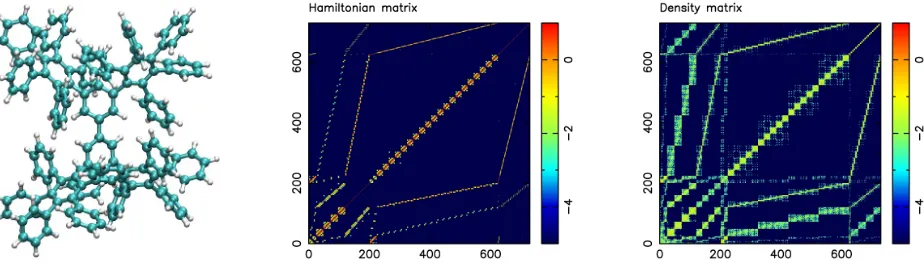
Figure 1: Molecular representation of phenyl dendrimer (left) using cyan and white spheres for carbon and hydrogen atoms, respectively. Hamiltonian matrix as 2D representation (middle) and thresholded density matrix (right). All plots show log10 of the absolute values of all matrix
[image:9.612.83.529.377.492.2]ele-ments. The SM-SP2 algorithm was used to compute the density matrix. Figure taken from Djidjev et al. (2016). Copyright c2016 Society for Industrial and Applied Mathematics. Reprinted with permission. All rights reserved.
Table 1: Physical systems of our study: number of vertices n in the graph and number of edges m. Table taken from Djidjev et al. (2016). Copyright c2016 Society for Industrial and Applied Mathematics. Reprinted with permission. All rights reserved.
Name n m m/n Description
polyethylene dense crystal 18432 4112189 223.1 crystal molecule in water solvent (low threshold) polyethylene sparse crystal 18432 812343 44.1 crystal molecule in water solvent (high threshold)
phenyl dendrimer 730 31147 42.7 polyphenylene branched molecule
polyalanine 189 31941 1879751 58.9 poly-alanine protein solvated in water
peptide 1aft 385 1833 4.76 ribonucleoside-diphosphate reductase protein
polyethylene chain 1024 12288 290816 23.7 chain of polymer molecule, almost 1-dimensional polyalanine 289 41185 1827256 44.4 large protein in water solvent
peptide trp cage 16863 176300 10.5 smallest protein with ability to fold (in water)
urea crystal 3584 109067 30.4 organic compound in living organisms
A dendrimer molecule with 22 covalently bonded phenyl groups of solely C and H atoms is schematically shown in Figure 1 (left). The graph of the dendrimer molecule has 730 vertices, composed of 262 atoms and 730 orbitals.
Figure 1 (middle) displays the absolute values of the Hamiltonian matrix for the dendrimer system. Figure 1 (right) displays the density matrix encoding the physical properties of the system, which is obtained by applying the SM-SP2 algorithm to the Hamiltonian.
We threshold the density matrix at 10−5 to convert it into a graph needed to find meaningful physical components via graph partitioning. This is done with all systems of Table 1 to arrive at their adjacency matrices. The first column of Table 1 displays the molecule name, the number of vertices n and edges m (second and third column) of its graph representation, and its average vertex degree m/n (fourth column). A short description of the molecule can be found in the last column.
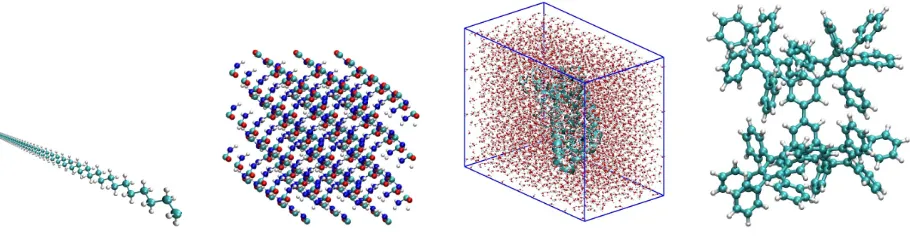
Figure 2: Molecular systems of this study: polyethyene linear chain (first plot), urea crystal (second plot), 189 residue polyalanine solvated in a water box (third plot), and phenyl dendrimer molecule (fourth plot). Cyan, blue, red and white spheres represent carbon, nitrogen, oxygen and hydrogen atoms, respectively. Figure taken from Djidjev et al. (2016). Copyright c2016 Society for Industrial and Applied Mathematics. Reprinted with permission. All rights reserved.
Figure 2 displays a one dimensional system in the first panel (polyethyene linear chain with repeated CH2 units), an anisotropic pristine 3D urea crystal (second panel), a polyalanine molecule solvated
in water (third panel) with a typicalα-helix secondary structure, and a dendrimeric system with a fractal arrangement of phenyl rings (fourth panel) to challenge our partitioning algorithms.
4.3 Comparison of the Partitioning Algorithms
Six methods are tested to partition each graph of Table 1 into 16 parts:
1. METIS with parameters of Section 4.1;
2. METIS with subsequent simulated annealing (SA);
3. hMETIS;
4. hMETIS with subsequent SA;
5. KaHIP;
6. KaHIP with subsequent SA.
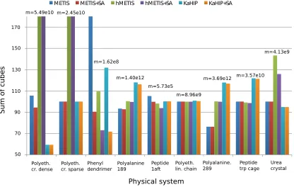
As before, the sum of cubes (3) criterion is used to assess the effectiveness of each method. Figures 3 and 4 show experimental results. We observe that all algorithms perform well (with the exception of the first two systems), and thatMETIS and KaHIP are significantly faster than
hMETIS. Importantly, post-processing with SA seems to improve solutions in almost all cases at negligible additional runtime, and is thus recommended.
Surprisingly, CH-partitions seem to pose a challenge for hMETIS as its solutions are usually worse than those of the other two methods, and its runtime significantly exceeds the one of the other methods (an explanation of this remains for further reseach). We conclude that for these two reasons,hMETIS seems unsuited for QMD simulations over longer time intervals, which is the aim of this work.
Figure 3: Sum of cubes performance measure to evaluate partitions. Values are normalized to have a median of 100. To make the chart more informative, very large values are truncated, though all exact values can be found in (Djidjev et al., 2016, Table 2). Figure taken from Djidjev et al. (2016). Copyright c2016 Society for Industrial and Applied Mathematics. Reprinted with permission. All rights reserved.
The behavior of our algorithms seems to be dependent on the sparsity of the graph of a physical system. First, METIS is able to outperform hMETIS for denser graphs, but not for sparser ones. Second, the post-improvement of partitions with SA seems to be especially effective for dense graphs, which can be explained with the fact that dense graphs offer more possibilities to reassign and optimize edges than sparse graphs. This can be seen when applying the combination of METIS+SAto the dense dendrimer system, see (Djidjev et al., 2016, Table 2) for details.
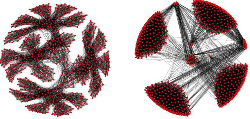
Figure 5 visualizes the relationship between the graph structure of a molecule (for the phenyl dendrimer molecule of Table 1) and its graph partitioning obtained through METIS and SA. After partitioning the molecular graph structure, the fractal-like structure of the phenyl dendrimer molecule and its dense components become clearly visible, as well as its sparse connections to other dense components. This structure is what our algorithm exploits to reduce the computations of the density matrix. Interestingly, SA sometimes dissolves entire partitions (meaning it produces partitions with no vertices), since such imbalanced partitions still yield a further decrease of the objective function (3).
4.4 Parallelized Implementation of G-SP2
Figure 4: Computing time for partitioning. Test systems of Table 1. We use the formatting of Figure 3 to handle the big discrepancy between values for different graphs. Figure taken from Djidjev et al. (2016). Copyright c2016 Society for Industrial and Applied Mathematics. Reprinted with permission. All rights reserved.
In particular, to measure the speed-up, we run METIS and METIS+SA on the polyalanine 259 protein system of Table 1 and record the obtained CH-partitions. Computations were carried out with the Wolf IC cluster of Los Alamos National Laboratory, whose computing nodes have 2 sockets each containing an 8-core Intel Xeon SandyBridge E5-2670, amounting to a total of 16 cores per computing node. A total of 32 GB of RAM are shared between the sixteen cores on each node, which are connected using a Qlogic Infiniband (IB) Quad Data Rate (QDR) network in a fat tree topology using a 7300 Series switch. Parallelization across nodes was done with OpenMPI, and parallelization across cores within a node was done with OpenMP.
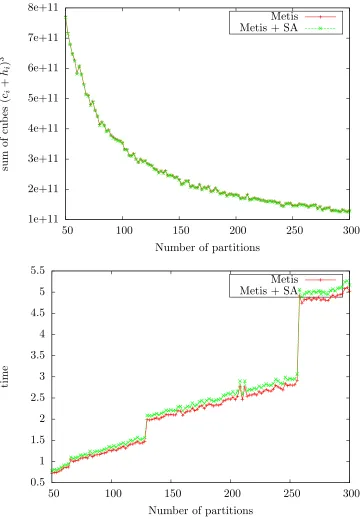
The sum of cubes measure and the computing time are displayed in Figure 6 as a function of the number of CH-partitions for thepolyalanine 259 protein system. We observe in Figure 6 (top) that the total effort of G-SP2, measured with the sum of cubes criterion, decreases monotonically as a function of the number of partitions and parallelized subproblems.
Figure 5: Left: Original graph extracted from the density matrix for the phenyl dendrimer molecular structure. Note the fractal-like structure of the graph. Right: Rearranged graph by the partitions resulting from the METIS + SA algorithms. Only edges with weights larger than 0.01 were kept to ease visualization.
algorithm decreases when applied in parallel despite the increasing effort to compute a partitioning.
4.5 Single Node SM-SP2 versus Parallelized Implementation of G-SP2
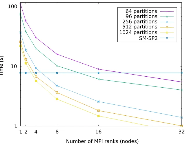
Figure 7 aims to quantify the computational savings over single node G-SP2 when running our proposed parallel SP2 algorithm. For this, Figure 7 compares the runtime for our parallel G-SP2 on 1−32 nodes against a threaded single node implementation of SM-SP2. This is due to the fact that the communication overhead exceeds the gain obtained by the extra computing power in a multi-node implementation, which is also the main motivation for developing G-SP2. As before, we employed METIS with parameters specified in Section 4.1 together with SA for post-processing. The test system is again the polyalanine 259 molecule.
Figure 7 shows that, as expected, both an increasing number of nodes and an increasing number of partitions decreases the G-SP2 runtime. When only few nodes are used for parallelization, the decrease in runtime is most pronounced since then, increasing the number of parallel nodes causes the runtime to drop sharply. For a higher number of nodes the curves somewhat flatten out.
1e+11 2e+11 3e+11 4e+11 5e+11 6e+11 7e+11 8e+11
50 100 150 200 250 300
sum
of
cub
es
(ci
+
hi
)
3
Number of partitions
Metis Metis + SA
0.5 1 1.5 2 2.5 3 3.5 4 4.5 5 5.5
50 100 150 200 250 300
time
Number of partitions
[image:14.612.123.487.114.633.2]Metis Metis + SA
100
10
Time [s]
1
1 2 4 8 16 32
[image:15.612.148.467.72.321.2]Number of MPI ranks (nodes) 64 partitions 96 partitions 256 partitions 512 partitions 1024 partitions SM-SP2
Figure 7: Runtime of parallelized G-SP2 as a function of the number of nodes. Different numbers of partitions. G-SP2 applied to the polyalanine 259 molecule. Figure taken from Djidjev et al. (2016). Copyright c2016 Society for Industrial and Applied Mathematics. Reprinted with permission. All rights reserved.
4.6 Relationship between Molecular System and Partitions
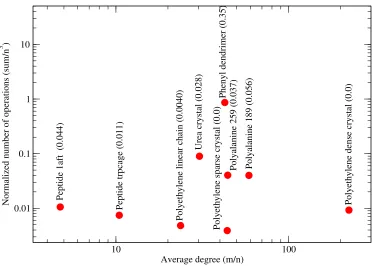
Figure 8 does not seem to exhibit a correlation between the molecular connectivity (measured with the average graph degree) and the normalized number of operations (NNO), defined as the sum of cubes criterion (3) normalized by the complexityn3 of the dense matrix-matrix multiplication. The observation also applies to the polyethylene dense crystal, whose normalized number of operations remains low although its average degree is high. Similar observations can be made for other molecules with a smaller average degree.
Our algorithm is capable of finding the lowest NNO for 1-dimensional systems such as the polyethylene linear chain and the polyethylene sparse crystal. According to Bunn (1939), regular agglomerates of polyethylene chains align along a particular direction with a large chain-to-chain distance. We conjecture that the reason for this lies in the sparsity of the system.
We do not observe any advantage of our approach (measured via NNO) for regular systems (polyethylene linear chain, polyethylene sparse crystal, polyethylene dense crystal and urea crystal). A difficult case for our graph partitioning task is the phenyl dendrimer (expressed through its high NNO values). This is due to the fractal-like structure of the graph associated with the molecule. According to (Djidjev et al., 2016, Table 2),METIS and SA together seem to yield the best runtime for this molecule.
10 100 Average degree (m/n)
0.01 0.1 1 10
Normalized number of operations (sum/n
3 )
Polyethylene dense crystal (0.0)
Peptide trpcage (0.011)
Polyethylene linear chain (0.0040)
Urea crystal (0.028)
Polyethylene sparse crystal (0.0)
Phenyl dendrimer (0.35)
Polyalanine 259 (0.037) Polyalanine 189 (0.056)
[image:16.612.121.498.67.333.2]Peptide 1aft (0.044)
Figure 8: Sum of cubes criterion (3) normalized by the complexity n3 of the dense matrix-matrix multiplication. Number of vertices n, number of edges m, and average degree m/n. Test systems of Table 1. Brackets show fractions of (max−min)/n(MMPN). For the combination METIS and SA similar trends are expected. Figure taken from Djidjev et al. (2016). Copyright c2016 Society for Industrial and Applied Mathematics. Reprinted with permission. All rights reserved.
denoted as max and min, respectively. The conjectured correlation is clearly visible in Figure 8: the dendrimer tends to both large MMPN and NNO values, proteins exhibit intermediate values of both MMPN and NNO and finally, we observe low values of both MMPN and NNO for sparse ordered systems such as polyethyene chains.
5
Discussion
This paper speeds up the computation of the density matrix in MD simulations through paralleliza-tion, informed by graph partitioning applied to the structure graph underlying a molecule. Our experimental results are based on graphs derived from density matrices of physical systems.
In our article we focus on a certain flavor of the classical graph partitioning problem arising from molecular dynamics simulations. In contrast to classical edge cut partitioning, we minimize partitions with respect to both the number of their core vertices and the number of their neighbors in adjacent partitions (halos). To the best of our knowledge, this type of graph partitioning (which we coin CH-(core-halo)-partitioning) has not been studied previously.
computational runtime. Special focus is given to the post-processing of partitions obtained with conventional graph partitioning algorithms for which we use our own modified SA approach.
We find that our flavor of the partitioning problem can be solved using standard graph parti-tioning packages. Moreover, post-optimization of the partitions obtained through classical graph partitioning packages can be performed well with our SA scheme. As expected, the time to evaluate matrix polynomials for different system (graph) sizes decreases with both the number of processors and parts in our simulations. Our main result is that the increased effort for graph partitioning and post-optimization with SA is beneficial overall when applying our parallelized version of the G-SP2 algorithm to meaningful physical systems. Based on our observation that METIS with a SA post-processing step is significantly faster than competing methods while giving the best results on average, we recommend this combination for practical use.
References
Aleksandrov, L. and Djidjev, H. N. (1996). Linear algorithms for partitioning embedded graphs of bounded genus. SIAM J. Discrete Math., 9(1):129–150.
Bader, D. A., Meyerhenke, H., Sanders, P., and Wagner, D., editors (2013). Graph Partition-ing and Graph ClusterPartition-ing - 10th DIMACS Implementation Challenge Workshop, volume 588 of
Contemporary Mathematics. AMS.
Bock, N. and Challacombe, M. (2013). An optimized sparse approximate matrix multiply for matrices with decay. SIAM Journal on Scientific Computing, 35(1):C72–C98.
Borstnik, U., VandeVondele, J., Weber, V., and Hutter, J. (2014). Sparse matrix multiplication: The distributed block-compressed sparse row library. Parallel Computing, 40:47–58.
Bunn, C. (1939). The crystal structure of long-chain normal paraffin hydrocarbons. The ”shape” of the CH2 group. Trans. Faraday Soc., 35:482–491.
Djidjev, H. N., Hahn, G., Mniszewski, S. M., Negre, C. F., Niklasson, A. M., and Sardeshmukh, V. (2016). Graph partitioning methods for fast parallel quantum molecular dynamics (full text with appendix).SIAM Workshop on Combinatorial Scientific Computing (CSC16). arXiv:1605.01118, pages 1–17.
Elstner, M., Porezag, D., Jungnickel, G., Elsner, J., Haugk, M., Frauenheim, T., Suhai, S., and Seifert, G. (1998). Self-consistent-charge density-functional tight-binding method for simulations of complex materials properties. Phys. Rev. B, 58(11):7260–7268.
Fiduccia, C. and Mattheyses, R. (1982). A linear time heuristic for improving network partitions.
In Proc. 19th IEEE Design Automation Conference, pages 175–181.
Finnis, M. W., Paxton, A. T., Methfessel, M., and van Schilfgarde, M. (1998). Crystal structures of zirconia from first principles and self-consistent tight binding. Phys. Rev. Lett., 81:5149.
Ford Jr., L. and Fulkerson, D. (1956). Maximal flow through a network.Canad. J. Math., 8:399–404.
Hendrickson, B. and Leland, R. (1995). A Multi-Level Algorithm For Partitioning Graphs. Pro-ceedings of the IEEE/ACM SC95 Conference.
Karypis, G. and Kumar, V. (1998). A hypergraph partitioning package.
Karypis, G. and Kumar, V. (1999). A fast and high quality multilevel scheme for partitioning irregular graphs. SIAM J. Sci. Comput., 20(1):359–392.
Karypis, G. and Kumar, V. (2000). Multilevel k-way hypergraph partitioning. VLSI Design, 11(3):285–300.
Kernighan, B. W. and Lin, S. (1970). An efficient heuristic procedure for partitioning graphs. Bell Sys. Tech. J., 49(2):291–308.
Kirkpatrick, S., Gelatt Jr, C., and Vecchi, M. (1983). Optimization by simulated annealing.Science, 200(4598):671–680.
Lipton, R. J. and Tarjan, R. E. (1979). A separator theorem for planar graphs. SIAM Journal on Applied Mathematics, 36(2):177–189.
Miller, G. (1997). Separators for sphere-packings and nearest neighbor graphs.
Mniszewski, S. M., Cawkwell, M. J., Wall, M., Moyd-Yusof, J., Bock, N., Germann, T., and Niklasson, A. M. (2015). Efficient parallel linear scaling construction of the density matrix for born-oppenheimer molecular dynamics. J Chem Theory Comput, 11(10):4644–4654.
Niklasson, A. M. (2002). Expansion algorithm for the density matrix.Phys. Rev. B, 66(15):155115– 155121.
Niklasson, A. M., Mniszewski, S. M., Negre, C. F., Cawkwell, M. J., Swart, P. J., Mohd-Yusof, J., Germann, T. C., Wall, M. E., Bock, N., Rubensson, E. H., and Djidjev, H. N. (2016). Graph-based linear scaling electronic structure theory. J Chem Phys, 144(23):234101.
Sanders, P. and Schulz, C. (2011). Engineering multilevel graph partitioning algorithms. InLNCS, volume 6942, pages 469–480.
Sanders, P. and Schulz, C. (2013). Think Locally, Act Globally: Highly Balanced Graph Parti-tioning. InInternational Symposium on Experimental Algorithms (SEA), volume 7933 ofLNCS, pages 164–175. Springer.
VandeVondele, J., Bortnik, U., and Hutter, J. (2012). Linear scaling self-consistent field calculations with millions of atoms in the condensed phase. Journal of Chemical Theory and Computation, 8(10):3565–3573. PMID: 26593003.
Walshaw, C. and Cross, M. (2000). Mesh Partitioning: A Multilevel Balancing and Refinement Algorithm.
A
Proofs for Section 2
For any graphIand vertexv∈I, theneighborhood ofvinIis the setN(v, I) ={w∈V(I)|(v, w)∈ E(I)}. LetH =P(G),v be a vertex ofG, and Hv denote the subgraph ofH induced byN(v, H).
For the following lemmas we assume thatTi∩E(H) =∅for alli, i.e., none of the edges inH=P(G)
are thresholded. We have the following properties.
Lemma 2. Let v be a vertex of G. Then N(v,P(G)) =N(v,P(Hv)).
Proof. First we prove that N(v,P(G)) ⊆ N(v,P(Hv)). Let w ∈ N(v,P(G)). Then (v, w) ∈
E(P(G)) and hence (v, w) ∈ E(Hv) ⊆ E(H). Since by assumption Ti∩E(H) = ∅, (v, w) 6∈ Ti
for all i. From (v, w) ∈ E(Hv), the last relation, and the fact that all vertices of H have loops,
(v, w)∈E(P(Hv)). Hence, w∈N(v,P(Hv)).
Now we prove that N(v,P(Hv)) ⊆ N(v,P(G)). Let w ∈ N(v,P(Hv)). Since P(Hv) and Hv
have the same vertex sets, we have w ∈ N(v, Hv). Furthermore, since Hv is a subgraph of H,
w∈N(v, H) =N(v,P(G)).
The lemma shows thatv has the same neighbors in P(G) and P(Hv), i.e., their corresponding
matrices have nonzero entries in the same positions in the row (or column) corresponding tov. We will next strengthen that claim by showing that the corresponding nonzero entries contain equal values.
Let Xv be the submatrix of A defined by all rows and columns that correspond to vertices of
V(Hv). We will call vertexv thecoreand the remaining vertices the halo ofV(Hv). We define the
set{V(Hv)|v∈G} to be theCH-partition ofG. Note that, unlike other definitions of a partition
used elsewhere, the vertex sets of CH-partitions (and, specifically, the halos) can be, and typically are, overlapping.
Lemma 3. For anyv∈V(G) and any w∈N(v,P(G)), the element ofP(A)corresponding to the
edge (v, w) of P(G) is equal to the element of P(Xv) corresponding to the edge (v, w) of P(Hv).
Proof. Let m = 2s be the degree of P. We will prove the lemma by induction on s. Clearly, the
claim is true fors= 0 since the elements of bothA1 andX1 are original elements of the matrixA. Assume the claim is true fors−1. DefineP0 =P1◦T1◦. . .◦Ps−1◦Ts−1. By the inductive assumption,
the corresponding elements in the matrices A0 = P0(A) and X0 = P0(X) have equal values. We need to prove the same for the elements ofA02 andX02.
Let (v, w) ∈ E(P(G)). By Lemma 2, (v, w) ∈ E(P(Hv)). For each vertex u of P(Hv) let u0
denote the corresponding row/column ofX. We want to show thatP(A)(v, w) =P(X)(v0, w0). By definition of matrix product, A02(v, w) = P
A0(v, u)A0(u, w), where the summation is over all u such that (v, u),(u, w) ∈ E(P(G)). Similarly, X02(v0, w0) = P
X0(v0, u0)X0(u0, w0), where the summation is over the values of u0 corresponding to the values of u from the previ-ous formula, by Lemma 2. By the inductive assumption, A0(v, u) = X0(v0, u0) and A0(u, w) = X0(u0, w0), thus A02(v, w) = X02(v0, w0). Since by assumption A0(v, w) = X0(v0, w0), we have Ps(A0)(v, w) = Ps(X0)(v0, w0), and hence P(A)(v, w) = (Ps◦Ts)(A0)(v, w) = (Ps◦Ts)(X0)(v0, w0) =
P(X)(v0, w0).
Lemma 3 implies the following algorithm to computeP(A) given we know its sparsity structure inHv:
2. For the i-th part Πi of Π whose core is the i-th vertex of G(A), construct a submatrix Ai
containing the rows and columns of Acorresponding to the vertices of Πi;
3. Compute P(Ai) for all i;
4. Define P(A) as a matrix whosei-th row has nonzero elements corresponding to thei-th row of P(Ai) (subject to appropriate reordering).
Clearly, in many cases it will be advantageous to consider CH-partitions whose cores contain multiple vertices. We will next show that the above approach for CH-partitions with single-node cores can be generalized to the multi-node core case.
We will generalize the definitions ofN(v,P(G)) andN(v,P(Hv)) for the case where the vertex
v is replaced by a set U of vertices of G. For any graph I, we define N(U, I) = S
v∈UN(v, I).
Furthermore, we define by HU the subgraph of H induced by N(U, H).
Suppose the sets {Ui | i= 1, . . . , q} are such that SiUi = V(G(A)) and Ui ∩Uj =∅. In this
case we can define a CH-partition of G=G(A) consisting ofq sets, where for eachi,Ui is the core
and N(Ui, H)\Ui is the halo of Πi.
The following generalizations of Lemma 2 and Lemma 3 follow in a straightforward manner.
Lemma 4. Denote byHi the subgraphP(HUi) of G. Let v be a vertex of Ui. Then N(v,P(G)) =
N(v, Hi).
Denote by AUi the submatrix of A consisting of all rows and columns that correspond to
vertices of V(HUi). The following main result of this section shows that P(A) can be computed
on submatrices of the Hamiltonian: this insight justifies the parallelized evaluation of a matrix polynomial.
Lemma 5. For any v ∈Ui and any w ∈ N(v,P(G)), the element of P(A) corresponding to the
edge (v, w) of P(G) is equal to the element of P(AUi) corresponding to the edge (v, w) of Hi.
In case of a QMD simulation, as outlined in Section 2, we assume that the sparsity structure of P(A) can be approximated by the one of the density matrix Dfrom the previous QMD simulation step. For the halos we approximate H =P(G) with G(D) as before, and use the current H as a substitute for the halos. This leads to the generalization of the partitioned algorithm for computing P(A) in case of multi-vertex cores given at the end of Section 2.
B
Further Details on Experimental Results
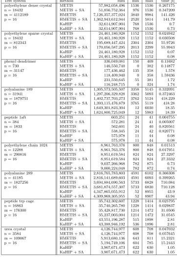
Table 2: Various test systems (first column) evaluated by different partition schemes (second col-umn; number of vertices n, edgesm, and partitionsp are given). Results measured with the sum of cubes (3) criterion (sum), the sum of size and halo for the smallest CH-partition (min) as well as the biggest CH-partition (max), and the overall runtime (in seconds) are given in columns 3-6.
Test system method sum min max time [s]
polyethylene dense crystal METIS 57,982,058,496 1536 1536 0.267175
n = 18432 METIS + SA 51,856,752,364 976 1536 0.347209
m = 4112189 HMETIS 7,126,357,377,024 3840 9984 141.426
p = 16 HMETIS + SA 1,362,943,612,944 2520 5814 141.79
KaHIP 32,614,907,904 768 1536 0.7
KaHIP + SA 32,614,907,904 768 1536 0.73
polyethylene sparse crystal METIS 24,461,180,928 1152 1152 0.024942
n = 18432 METIS + SA 24,461,180,928 1152 1152 0.030508
m = 812343 HMETIS 195,689,447,424 2304 2304 55.9726
p = 16 HMETIS + SA 170,056,587,295 2013 2299 55.9943
KaHIP 24,461,180,928 1152 1152 0.07
KaHIP + SA 24,461,180,928 1152 1152 0.08
phenyl dendrimer METIS 336,049,081 150 409 0.13482
n = 730 METIS + SA 146,550,740 0 382 0.14877
m = 31147 HMETIS 177,436,462 135 358 1.578
p = 16 HMETIS + SA 118,409,940 0 358 1.59436
KaHIP 231,550,645 55 381 1.72
KaHIP + SA 116,248,715 0 324 1.74
polyalanine 189 METIS 1,305,573,505,507 3358 5145 0.332091
n = 31941 METIS + SA 1,297,206,329,828 3362 5093 0.372463
m = 1879751 HMETIS 1,402,737,703,273 3762 5124 418.229
p = 16 HMETIS + SA 1,393,115,476,879 3765 5119 418.28
KaHIP 1,649,301,823,304 12 6030 18.35
KaHIP + SA 1,624,800,725,049 12 5983 18.39
peptide 1aft METIS 603,251 24 41 0.004755
n = 384 METIS + SA 572,281 24 41 0.005007
m = 1833 HMETIS 562,601 24 40 0.820561
p = 16 HMETIS + SA 538,345 24 42 0.820771
KaHIP 575,978 11 44 0.08
KaHIP + SA 575,978 11 44 0.08
polyethylene chain 1024 METIS 8,961,763,376 800 848 0.01513
n = 12288 METIS + SA 8,961,763,376 800 848 0.017951
m = 290816 HMETIS 8,951,619,584 824 824 27.3297
p = 16 HMETIS + SA 8,951,619,584 824 824 27.3332
KaHIP 9,037,266,968 782 875 0.73
KaHIP + SA 9,000,224,048 782 872 0.74
polyalanine 289 METIS 2,816,765,783,803 4591 6102 0.366308
n = 41185 METIS + SA 2,816,141,689,603 4591 6093 0.399265
m = 1827256 HMETIS 3,694,884,690,563 5733 6828 710.084
p = 16 HMETIS + SA 3,681,874,557,307 5733 6830 710.128
KaHIP 4,347,865,055,912 52 8955 43.9
KaHIP + SA 4,309,969,305,955 52 8907 43.94
peptide trp cage METIS 35,742,302,607 1228 1414 0.025795
n = 16863 METIS + SA 35,740,265,780 1228 1414 0.029837
m = 176300 HMETIS 35,428,817,730 1214 1472 31.0506
p = 16 HMETIS + SA 35,237,003,004 1214 1472 31.0545
KaHIP 43,551,196,287 515 1898 2.81
KaHIP + SA 43,388,946,192 536 1896 2.81
urea crystal METIS 4,126,744,977 608 708 0.047032
n = 3584 METIS + SA 4,126,744,977 608 708 0.057645
m = 109067 HMETIS 5,913,680,136 643 811 15.2321
p = 16 HMETIS + SA 5,194,749,106 604 785 15.2443
KaHIP 3,907,671,473 622 630 1.05