An Output Stabilization Problem of Distributed Linear Systems Approaches and Simulations

(1)

An Output Stabilization Problem of Distributed Linear

Systems Approaches and Simulations

El Hassan Zerrik, Yassine Benslimane

Department of Mathematics and Computer Science, Faculty of Science, University of Moulay Ismaïl, Meknès, Morocco

Email: {zerrik3, bensyassine}@yahoo.fr

Received February 13, 2012; revised March 20, 2012; accepted March 28, 2012

ABSTRACT

The goal of this paper is to study an output stabilization problem: the gradient stabilization for linear distributed systems. Firstly, we give definitions and properties of the gradient stability. Then we characterize controls which stabilize the gradient of the state. We also give the stabilizing control which minimizes a performance given cost. The obtained re-sults are illustrated by simulations in the case of one-dimensional distributed systems.

Keywords: Distributed System; Gradient Stability; Gradient Stabilization; Stabilizing Control

1. Introduction

One of the most important notions in systems theory is the concept of stability. An equilibrium state is said to be stable if the system remains close to this state for small disturbances; and for an unstable system the question is how to stabilize it by a feedback control.

For finite dimensional systems, the problem of stabili-zation was considered in many works and various results have been developed [1]. In the infinite dimensional case, the problem has been treated in Balakrishnan [2], Curtain and Zwart [3], Pritchard and Zabczyk [4], Kato [5], Trig- giani [6]. Many approaches have been considered to characterize different kinds of stabilization for linear distributed systems: Lyapunov and Riccati equation for exponential stabilization, and dissipative type criterion for the case of strong stabilization [3-5,7]. The problem has been also treated by means of specific state space decomposi-tion [6]. The above results concern the state, but in many real problem the stabilization is considered for the state gradient of the considered system, which means to find a feedback control such that the gradient 0, when

. t 

For example the problem of thermal insulation where the purpose is to keep a constant temperature of the sys-tem with regards to the outside environment assumed to be with fluctuating temperature. Thus one has to regulate the system temperature in order to vanish the exchange thermal flux. This is the case inside a car where one has to change the level of the internal air conditioning with respect to the external temperature.

As we cannot always have external measurements, we

use a sensor to measure the flux, which is a transducer producing a signal that is proportional to the local heat flux.

The purpose of this paper is the study of gradient sta-bilization. It is organized as follows: In the second sec-tion we define and characterize gradient stability. In the third section, we characterize gradient stabilizability, by finding a control that stabilizes the gradient of a linear distributed system and we give characterizations of such a control. In the fourth section we search the minimal cost control that stabilizes the system gradient. In the last section we give an algorithmic approach for control im-plementation and simulation examples.

2. Gradient Stability

This section is devoted to some preliminaries concerning definition and characterization of gradient stability for linear distributed systems.

2.1. Notations and Definitions

m

I

Let  be an open regular subset of R and let us

consider the state-space system

 

0 0

z Az t

z z H



 _

  

 _ _ (1) 

 

: A

where D A HH

 

S t t0

is a linear operator gener-ating a strongly continuous semigroup , , on the state space H which is continuously embedded in

 

1

(2)

H is endowed with its a complex inner product , .

and the corresponding norm .



 





. We define the operator by:

2

1 2

, , ,

m

z z z

:H L

z

x x x

       _     

 



_L2 _



m

 

 

(2)

is endowed with its usual complex inner product , _m and the corresponding norm ._m where:

 







 







   

2 2 1 .,. , d m m i m i i i

L L C

f g f x g x x

I       

 

 1 2 (3)

With f 



f, , ,f  fm



and g



g g1, 2, , gm





*

G  

 0,1, , .

i  m

 

0

S t z

where The mild solution of (1) is

given by

 

.

 

 

z t 

2

,

i i

f g L

*



Let denote the adjoint operator of , and we define the operator which a bounded operator applying H into itself.

Definition 2.1

The system (1) is said to be

 Gradient weakly stable (g.w.s) if  z0 H, the

cor-responding solution z t

 

of (1) satisfies

 

_,



2

 



m

y L

  

, 0 as

m

z t y t

  

 Gradient strongly stable (g.s.s) if for any initial con-dition z0H the corresponding solution z t

 

of

(1) satisfies:

 

0 as t

  

m

z t 

 Gradient exponentially stable (g.e.s) if there exist M,

0

  such that:

 

0 , 0,z0H

 

t m

z t Me z t

 

Remark 2.2

From the above definitions we have: 1) g.e.s g.s.s g.w.s.

2) If the system (1) is stable then it also gradient sta-ble.

3) We can find systems gradient stable but not stable. This is illustrated in the following example.

Exemple 2.3

Let  

 

0,1 , on we consider the following

system

 

1 H 

 

1 0 1, 0

t Az t

z z

t t

z z H

 _ _     

 

0, .,0 z t   _         (4)

Where Az  z z and

2 2

d dx

 s the Laplace op-erator.

 i



The eigenpairs  i, i



,iIN

 

of A are given by:

 

2

1 π 0

2 _cos _π ₀

1 π

i

i i

x i x i

i         _ _  _ 



A generates a strongly continuous semigroup S t



given by

 

0 0

0

eit ,

i i

i

S t z  z  







0 0

 

 

then (4) isn’t stable but

1

2 2 2 2

0 0 0 2 2 0 e , e t

i i m

m i t

S t z z

z         



Therefore the system (4) is g.e.s. 2.2. Characterizations

The following result links gradient stability of the system (1) to the spectrum properties of the operator A.

Let us consider the sets



 





 



1 _{, Re} _0,

A A N A I N G

       

and



 





 



2 _A _A _{, Re} _0,_{N A} _I _{N G}

       

 

A



where  and N A



 

1 _.

A

  

are the points spectrum and the kernel of the operator A.

Proposition 2.4

1) If the system (1) is g.w.s then

2) Assume that the state space H has an orthonormal

basis

 

n _n

 

1

A



 of eigenfunctions of A, if   0

and,

for some _Re

 

2

 

_,

A

 ,

   for all  

 

then the system (1) is g.e.s.

Proof

A

1) Assume that there exists   such that

 

Re  0 and there exists H such that A  .

 

et

S t 

0

z

For , the solution of (1) is  

 

_, _eRe t 2 2 ₀, so

m m

m

S t     

      

0

z H

hence the system (1) is not g.w.s.  we have 2) For

 

0 0 , ,

0 1

en n ,

r t

n k n k

n k

S t z  z  

 

 

 



n

r _n.

where is the multiplicity of the eigenvalue 

 

1 _,

A

  gives:

 

0 e 0

t m

S t z M  z

(3)

for some M 0.

So we have the g.e.s of the system (1).

As example we consider (4). We have: 1

 

A

  

and 2

 

A

 

  , Re , then the system (4)

is g.e.s.

 

1







2 _0, _;

2

π  

For the gradient exponential stability, we need the fol-lowing lemma.

Lemma 2.5

Assume that there exists a function

 

M t L  IR such that:





 

s t s, 0

 



S t



t0

S t s M t S

    (5)

Then the operators are uniformly bounded. Proof

Let us show that

 

0 sup t S t   





. Otherwise there exists a sequence t1k , t10 and k   such

that S t



1k



is increasing without bound.

Now we have:





2

 

0 k

k _m

S s z s



 

  



2

d d

m

S s z s



k 





and the right-hand side goes to zero when . By Fatou’s lemma liminf S s _k 0

m z



  

k  0 s

when , almost everywhere   

0 1

.

Hence for some s t we can find a subsequence

n k

 such that lim



₀



n S s kn z_m 0.

But with (5) we have



1 kn



_m



1 0







S t  z M t s S s

     ₀ k_n 0

m z



 

, n 

when which is a contradiction.

The conclusion follows from the uniform boundedness principle.

Proposition 2.6

Assume that (5) is satisfied and

 

n_{   }_0, _n _IN*

S nt S t t

   (6)

Then the system (1) is g.e.s if and only if

 

2

0 m

S t z







dt  ,z H

Proof

 





 

2 2 0 2 0 2 0 2

( ) d

d ( ) from lemm = a (3 t m m t m t

t S t z S t z s

S s t s z

M s S t s

N z          



2

d from (5)

.2)

m

s

z s

0

N ln S t





0

where , then    t t₀

0 0,

t 

 

, for some

hence 0 ₀ ln inf 0 t S t w t    

 

0 ln lim t S t w t     

 

Now we show that .

1

0,

sup ,

t t

N S t



  n IN

Let t1 > 0, and there exists 





1 1 1

nt  t n t for each tt₁, then

such that

 

1



1



ln S t ln S nt ln S t nt

t t t

  

 

With (4) we have

 

₁

 

1 1

ln S t nt ln S t _lnN

t t t t

     Therefore

 

0 ln l

limsup inf n liminfln

t t

t

S t S t S t

t  t  t

     

 

0 ln lim t S t w t   

then .



0, 0



,

Hence for all   there exists M' such that

 

e t ,

m

S t z M z

   z H, t0.

0 t

So the system (1) is g.e.s.

The converse is immediate. Example 2.7

The system (2) satisfies the conditions (5) and (6). In-deed:

 

1

z H

Let , and   .

 

We have

0

eit ,

i i

i

S t z  z 



 



 , which implies

 

1

2 2 2 2

0 2 2 e , e t

i i m

m i t

S t z z

z         



 

_e21t_. m

S t 

 

 

we can show that

2

0

d m

S t z t



We have

_

  .

Therefore the system (4) is g.e.s. Corollaire 2.8

Under conditions (5) and (6) and assume, in addition, that there exists a self-adjoint positive operator PL H

 

such that:

 

, , , 0,

Az Pz  Pz Az  Rz z  zD A (7)

 

RL H is a self-adjoint operator satisfying

where

2

, _m, for some 0

(4)

 

D A in H, and the continuity of

then (1) is g.e.s. Proof

We define the function V z

 

 Pz,z ,  z H.

 

z t S t and

For z₀D A

 

, we have z₀

 





 





 

0, 0,

V z t z S t ₀ z AS ₀

0 0

d d

,

t PAS z PS t t z

t

RS t z S t z

 

 

Thus

 

0,

 

0 dsV z

 

0 By (8), we ob- 0

RS s z S s z





tain

 

0 2 0

d m

S t z s



Sin

  .

ce



 

D A is dense H we can extended this

ine-z H

in

quality to all 0 , and the proposition 3.3 gives the

conclusion.

For the gradient strong stability we have the following result.

Proposition 2.9 Assume that the equation

 

, 0,

, ,

Az Pz  Pz Az  Rz z  zD A

has a self-adjoint positive PL H

 

, where

 

ing (8).

solution

RL H is a self-adjoint operator satisfy More-

over if the following condition holds

 

Re GAz z, 0,zD A (9)

then (1) is g.s.s.

r the function: Proof

Let us conside

 

, ,

V z  Pz z  z H

0

z D

For

 

A , we have z t

 

S t





z₀ and

 





 





 

0, 0,

V z S t z S ₀ z AS ₀

0 0

d d

,

t PA t z PS t t z

t

RS t z S t z

 

 

we obtain

 

0,

 

0 dsV z

 

₀ By (8),

0

RS s z S s z





 

2 0 0

d

m

S t z s



   and from (9), we have



 

2 0 _m 0.

S t z t



 

 Then

 

2

 

2

 

0 0

t t

m m

2 0

d d

m t z  



S t z s 



S t z s

We deduce

t S

 

2 0

0 for so

m S t z

z D A

 



 

0 _, _0,

me

z t t

z



 

(10)

From the density of

 

.

 , (10) is satisfied for all z0H. T

the gradient of (1) is strongly stable.

lizab

his means that

3. Gradient Stabi

ility

Let us consider the system

 

_{ }

0

z t

 

.,0 Az t

t  

 

 Bv t

H





(11)

with the same assumptions on A, and B is a bounded

lin-ear operator mapping U, the space of c

to be Hilbert space), into H.

Definition 3.1

z z

 _



ontrols (assumed

The system (11) is said to be gradient weakly (respec-tively strongly, exponentially) stabilizable if there exists a bounded operator KL H



,U



such that the system

  

  

z t

 

.,0 0

A BK z t

t z



 

    

(12)

z H

 

is g.w.s (respectively g.s.s, g.e.s). Remark 3.2

1) If a system is stabilizable, then it is also gradient stabilizable.

eaper than state stabi-liz if we consider the cost functional

 

2) Gradient stabilizability is ch ability. Indeed

2



0

and the spaces

d

v t t

q v 





2



_0, _;



_{; stabiliz the gradient}



ad

U  vL U v

and

es



2



_0, _;



_{; stabilizes the state .}



ad U v

Then we have 1

ad ad

U U and therefore

1

U  vL

 

₁

 

min min

ad ad

v U v U

q v q v

  

s a special

ca r

3) The gradient stabilization may be seen a se of output stabilization with output operato .

In the following we give the feedb k control which stabilizes the gradient of the system (11), by two ap-pr

position [6

3.

ac oaches.

The first is an extension of state space decom ] and the second one is based on algebraic Riccati equ-ation.

1. Decomposition Method

Let  0 be a fixed real and consider the subsets

 

s

 

u A

(5)

de-fined by

 



:

 

, Re

 



u A A

      

and

 



:

 

, Re

 



s A A

      

that _u

 

Assume  A is bounded and is separated

 

s

from the set  A in such a way that a rectifiable

curve can be drawn so as to enclose an g _s



sim op

ple closed

en set containin  A



in its interior and _u

 

A in

its exterior. This i e case, for example, where A is self-

adjoint with compact resolvent, there are at most finitely many nonnegative eigen ues of A and each with finite

dimensional eigenspace.

Then the state space H can be decomposed [5]

ac-cording to:

s th val

u s

HH H (13)

with Hu PH, Hs 



IP H



, and PL H

 

is the projection operator given by





1d

2π c

P I A

i

1 _  _



_



where C is a cl ed cuos rve surrounding s

 

A .

The system (11) may be decomposed into the two subsystems

 

_{ }

u u

0u 0

u u z t

A z t PBv t

t  

  

z Pz

 _

    

(14)

and

 

 

_{ }









0 0

s

s s

s

s z t



  

A z t t

z I P z

 

 

 

 _ _



   



IP Bv t

(15)

where As and Au are the restrictions of A to Hs and u

H , and are such that_s

 

A 

 

A_s , _u

 

A 

 

A_u ,

and Au is a bounded op

olu (

erator on Hu.

The s tions of 14) and (15) are given by

 

0 ₀

u u u u

z t S t z tS



t



PBv

 

 d (16

  

d P Bv

 

_

)

And

 

0 ₀





t

s s s s

z t S t z S t  I 

w

 

t and S_s

 

t denote th ion of

 (17)

 

_



here Su e restrict S t

 

to Hu and Hs, which are strongl inuous

rate u

y cont semi-groups gene d by A and A_s.

y r

For t stem state, it is known (see [6]) that if the operato

he s

s

A satisfies the spectrum growth assumption

 

_

_{ }

_

p s

ln

lim S ts su Re

t _t A

then stabilizing (11) comes back to stabilize (14).  (18)

The following proposition gives an extension of this result to the gradient case.

Proposition 3.3

3) and 

Let the state space satisfy the decomposition (1

s

A satisfy the following inequality

 

ln

lim S ts



 



sup Re s

t _t A

1) If the system (14) is gradient ex 

 (19)

ponentially (respec-tively strongly) stabilizable by a feedback control

u u

u K Gz





,



u

K

, with

 L H U , then the sys

gradient exponentially (respectively strongly) stabilizable us

tem (11) is ing the control v

 

u, 0 .

2) If the system (14) is gradient exponentially (resp strongly) stabilizab byle the feedback control: vK zu u,

with KuL H U



,



then the system (11) is gradient

exponentially (res gly) stabilizable using th

pectively stron e feedback operator K



Ku;0



.

Proof

We ve for the exponential case. In view of the above decomposition, we have:

gi the proof

 





sup Re  As  .

Hence if As satisfies (19) then for some M1 and



0,



 

  , we have: S ts M1e t

 

  , t0.

It follows that the system (15) is gradient exponen-tially stabilizable taking v(t) = 0.

Let Ku be uch that

 

eu 0

t

u u

z t  z , with

s F

 

u

u u u

F A PBK GL Z and there exists  0 2

su

, M > 0

ch that

 

2e 0

t

u _m u

z t M  z

 

Then with the feedback control vK Gz_u _u we have

 

3 e 0

t

u u

t  K  z 0

v M , with M 

From (17) and (18) we have 3

 

1e 0 3 0 e d

0

4 0

1 0

?

e e

t t s

u e

z



 

 

 _ 





with M40.

Thus the system (11) excited by

 

e t

s

M  z M

 

t s

s _m s u

t t

z t M  z M z  s

 

 

  

 

v t Kz t

satis-fies

 

1 4 2 0

e e

t t

z t M M M z

 

   

 

  

   _

 h shows that the system (11) is gradient exponen-tially stabilizable.

2) The case of strong stabilizability follows from si i- lar above techniques.

m _  

whic

 _

m Corollary 3.4

(6)

(13) and suppose that (19) is satisfied. If in addition 1) Hu is a finite dimensional space

2) The system (14) is controllable on Hu then the

sy dient exp tially stabilizable. trol-stem (11) is gra onen

Proof

The system (14) is of finite dimension and is con lable on the space Hu then it is stabilizable on the same

sp on

3.

ace, hence it is gradient stabilizable, the c clusion is obtained with the proposition 3.3.

2. Riccati Method

Let us consider the system (11) with the same assump-tions on A and B. We denote by K

 

ed

S t , t0 the

strongly continuous semigroup generat by ABK ,



,



where K is the feedback operator K L H

rato

U .

r such that (8) 

nt ope Let RL H

 

be a self-adjoi

is satisfied and suppose that the steady state Riccati equ-ation

 

* *

, , , ,

Az Pz  Pz Az  B Pz B Pz  Rz z 0, D A

(20)

*

z

has a self-adjoint positive solution PL H

 

, and let

K B P.

Proposition 3.5

1) If SK

 

t satisfies the conditions (5) and (6) e system (11) is gradient exponentially stabilizable by

 

, then th

the control *

 

_.

u t Kz t



2) If BK z z



, 0,zD A

 

then the system

(1 ngly stabilizable.

G A

1) is gradient stro

3) Suppose that the system (11) is gradient exponen-tially stabilizable. If in addition the feedback operator K

satisfies z c



A K z z



, ,zD A

 

,for some

c the state of the system (12) re

e th z D A

 

, we have

, Re

Gz B

> 0 then mains bounded.

Proof

The first and second points are deduced from the sec-ond section.

For th irst point: Let 0



    





1

 

2

Re ,

2

ABK z t z t  z t (21)

we obtain

t

 and from (21)



 

2



 

2 2



t

0 0

d 2

m c

z s s z t z

  



Since the system (11) is gradient exponentially stabi-

 

lizable then 2



0

d

m

z t t

  



, so there exists M 0

 

such that z t M, for all t0 and by the density

t Stabilization Control Problem Here we explore the control that stabilizes the gradient of

(11) as a s f the

(22)

of D A

 

in H we have the conclusion.

3.3. Gradien

the system olution o minimization prob-lem

 

minq v





ad vU



where q v

 

Rz t

   

,z t dt v t

 

2dt

 



_



_

with

0 0



  



2 0, ; ;q v



ad

U  vL U

and R is a linear bounded operator mapping H into itself

sfying (8).

classical result known for sta a-tion if Uad

 

and sati

We recall the te stabiliz

  for each initial state z0, then there

exists a unique control v that minimizes (22 nd giv-) a

en by v

 

t  B Pz t

 

where P is a positive solution

of the steady state Riccati Equation (20).

 

gr

If in addition the operator R is coercive then the state

of system (11) is exponentially stabilizable (see [7]). In the following we give an extension of the above re-sult to the adient case.

We suppose that Uad   for each initial state z H, and R satisfies (8).

Proposition 3.6

 

  

0

The control given by v t  B Pz t minimizes

 

q v where P assumed to be a self-adjoint, positive

operator, and satisfies the y state Riccati equation ), if in addition the sem oup S

 

t satisfies the

en th stead

(20 igr K

co e same control stabilizes the

gr P

t an algorithm which allows the ca n of the solution of problem (22) stabilizing the

gr is

control may be obtained by solving the algebraic Riccati nditions (5) and (6) th

adient of system (11) roof

The proof follows from [7], and the proposition 3.5.

4. Numerical Algorithm and Simulations

In this section we presen lculatio

adient of the system (11). By the previous result th Equation (20). Let Hn span e i



i, 1, 2, , n



where



e ii, 1



is a hilbertian basis of H. Hn is a subspace

of H endowed with the restriction of the inner product of H. The projection operator n:H Hn is defined by

 

1

,

n

n i

z e z e z H

 i i

 



 

The projection of (20) on space Hn, is given formally

by:

0

n n n n n n n n n

P A A P P B B P R  (23)

where An, Pn and Rn are respectively the projections

of A, P and R on Hn, and Bn the pr jection of B which

is mapping U the space of control in

o to Hn.

We have lim n n 0

(7)

verges to P strongly in H, (see [8]).

ojectio

We can write the pr n of (11) like

 

_{ }

n

n n n n n

z t

 

0 0

n

n n

A z t B B P z t

t

 

 

  

z



 z

(24)

xplicitly by:

 

0

n zn (25)

To calculate the matrix exponential we approximation with scaling and squaring (see [9]).

 

the solution of this system is given e

 

z t e



An B B P tn n n







use the Padé If we denote

 

 z t ,e , we have

 

1

n n i

i

z t z t e



 



  (26)

i

z_n t _n _i

n i

Let consider a time sequence tii , iN where 0

  small enough.

tion co

With these no nt stabiliza

e obtained s (Table 1

tations, the gradie ntrol

may b the algorithm step ).

Remark 4.1

The dimension of the projection space

be nsider

appro t.

n is choosing to

good approximation of the co ed system and priate for numerical constrain

Example 4.2 Let  [0,1], on

 

1 _{such that} ₀ ₁ ₀

d d

H z H

x x

_     _

 

which is an Hilbert space we consider the following sys-te

dz dz 



m

 

_{ }

 

2

0, 1,

1 1 ,0

2 3

D z t

Az t v t

t

z t z t

[0, ]

0 t 0

z x x x

 



 

  

 

   

 _  _  _

 _ _



(27)

0.

x x

  



 

where Az 02 z 0.5z , v t

 

H  t 0, D is

. ]

the restriction operator on D[02,0.9 , and w

 e

con-sider the problem (22) with R  

igroup .

inuous

A generates a strongly cont sem S t

 

given by:

 

0

, it

i i

e z

i

S t z   , where

01 i 

 



2

 

π 0.5 and 0.

i

   i

_{ }

x icos

_{ }

i xπ with

 

2

i  

 .

1 iπ

The state and the m (27) are unsta since ₀, ₁ 0

gradient of syste ble

   . Let consider the su



 i n x,  



Applying the algorithm taking the truncation at n = 5,

we obtain Figures 1 which illustrates the evolution of the system gradient and shows how the gradient evolves close to

gradient ilized with error equals 9.9836 ×

10 –4_{. This shows the}

effi-ciency of the developed algorithm.

In Table 2 we give the cost of gradient stabilizati of sy

bspace









1cos 1 π , 1

n i

H Span _ i x

zero when the time t increases.

The is stab

–7_{and cost equals 2.6982 × 10}

on stem (27) for different supports control “D”.

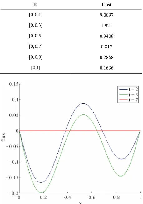
The Table 2 shows that there is relation between area of control support and the cost of gradient stabilization, more precisely more this area decreases more cost in-

Table 1. Algorithm.

1) Let 0 the threshold, n the dimension of the projection space, and zn 0 z₀n.

2) Solve (23) using Schur-type methods (see [10,11]) 3) Solve system (24) using formula (25) gives z tn i

4) Calculate z tn i by the formula (26).

[image:7.595.54.291.85.348.2]

5) If z tn i  stop, else 6) i = i + 1 and go to 3.

Table 2. Support control-cost stabilization.

D Cost

[0,0.1] 9.0097

[0,0.3] 1.921

0.9408

[0,0.7] 0.817

[ 0.1636

[0,0.5]

[0,0.9] 0.2868

[image:7.595.308.537.375.707.2]

0,1]

[image:7.595.309.538.377.704.2]

(8)

creases.

Example 4.3

Let  [0,1] on 1

 

0

H H  we consider the

(2 let boundary conditions: tem 7) with Dirich

 

_{ }

  

_,0 ₁



2 2

D z t

Az t v t

t

z x x x

 



 

  

 _{ }



[0, ]

x

 

 

(28)

where Az0.01 z 0.5z, v t

 

  H t 0, D[0, 0.3],

*

  . and we consi

The eige

der the problem npairs of A are

(22) with R

given by



 i, isin

 

i xπ



, 01 iπ

gradie (28) are unstable since 1 0

of system (28) for different zone control support “D”.

Also in this example, we remark that more the area of control support increases more the cost of gradient stabi-lization decreases.

4. Conclusions

In this paper the question of gradient stabilization is ex-plored. According to the conditions, satisfied by the dy-namic of system, and those satisfied by the state space, two methods are applied to characterize the controls of gradient stabilization namely, decomposition approach and Riccati method.

The obtained results are successfully illustrated by numerical simulations. Questions are still open, this is the case of regional gradient stabilization. It is under consid-eration and will be appear in separate paper.

he work presented here was carried out within the

sup-port of

Tech-nology.

REFERENCES

[1] W. M. Wonham, “Linear Multivariab rol: A Geo-metric Approach,” Springer-Verlag, Be

[2] A. V. Balakrishnan, “Strong Stabil e Steady State Riccati Equation,” Applied Mathematics and Opti- mization, Vol. 7, No. 1, 1981, pp. 3

doi:10.1007/BF01442125

1

i , with   i 0.

The state and the

 

2

0.5  . nt of system   .

We consider the subspace

 



sin π , 1, ,



n i

H   i x i  n with

 

2

1 iπ

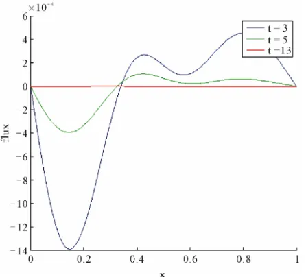
Applying the al

2

 .

gorithm with truncation (n = 5), the

evolution at times t = 3, 5,

an

[image:8.595.63.286.363.565.2]

i 

Figure 2 shows the gradient d 13.

In Table 3 we present the cost of gradient stabilization

gure 2. The gradient evolution for the Direchlet boundary F

co i

ndition case.

Table 3. Support control-cost stabilization.

D Cost

[0,0.1] 0.0247

5. Acknowledgements

T

the Academy Hassan II of Sciences and

le Cont rlin, 1974. izabity and th 35-345.

nd J. Zabczyk, “Stability and Stabilizabil- ity of Infinite Dimensional Systems,” SIAM Review, Vol.

pp. 25-51. doi:10.1137/1023003

[3] R. F. Curtain and H. J. Zwart, “An Introduction to Infi- nite Dimensional Linear Systems Theory,” Springer- Verlag, Berlin, 1995.

[4] A. J. Pritchard a 23, No.1, 1981,

[5] T. Kato, “Perturbation Theory for Linear Operators,” Springer-Verlag, Berlin, 1980.

[6] R. Triggiani, “On the Stabilizability Problem in Banach Space,” Journal of Mathematical Analysis and Applica- tions, Vol. 52, No. 3, 1979, pp. 383-403.

doi:10.1016/0022-247X(75)90067-0

[7] R. F. Curtain, and A. J. Pritchard, “Infinite Dimensional Linear Systems Theory,” Springer-Verlag, Berlin, 1978. [8] H. T. Banks and K. Kunisch, “The Linear Regulator

Problem for Parabolic Systems,” SIAM Journal on Con- trol and Optimization, No. 22, Vol. 5, 1984, pp. 684-696.

doi:10.1137/0322043

[0,0.3] 0.0039

[0,0.5] 0.0016

[0,0.7] 4.7255 × 10–4

[0,0.9] 2.6982 × 10–4

[0,1] 2.6081 × 10–4

g and Squaring Method for the [9] N. J, Higham, “The Scalin

Matrix Exponential,” SIAM Journal on Matrix Analysis and Applications, Vol. 26, No. 4, 2005, pp. 1179-1193.

doi:10.1137/04061101X

[image:8.595.59.286.620.732.2]

(9)

Vol. 24, No. 6, 1979, pp. 913-921.

doi:10.1109/TAC.1979.1102178

[11] W. F Arnold and A. J. Laub, “Generalized Eigenproblem