A linear time method for the detection of point and collective
anomalies
Alexander Fisch, Idris Eckley, and Paul Fearnhead
Lancaster University, United KingdomJune 7, 2018
Abstract
The challenge of efficiently identifying anomalies in data sequences is an important statistical problem that now arises in many applications. Whilst there has been substantial work aimed at making statistical analyses robust to outliers, or point anomalies, there has been much less work on detecting anomalous segments, or collective anomalies. By bringing together ideas from changepoint detection and robust statistics, we introduce Collective And Point Anomalies (CAPA), a computationally efficient approach that is suitable when collective anomalies are characterised by either a change in mean, variance, or both, and distinguishes them from point anomalies. Theoretical results establish the consistency of CAPA at detecting collective anomalies and empirical results show that CAPA has close to linear computational cost as well as being more accurate at detecting and locating collective anomalies than other approaches. We demonstrate the utility of CAPA through its ability to detect exoplanets from light curve data from the Kepler telescope.
1
Introduction
Anomaly detection is an area of considerable importance for many time series applications, such as fault detection or fraud prevention, and has been subject to increasing attention in recent years. See [4] and [25] for comprehensive reviews of the area. As [4] highlight, anomalies can fall into one of three categories: global anomalies, contextual anomalies, or collective anomalies. Global anomalies and contextual anomalies are defined as single observations which are outliers with regards to the complete dataset and their local context respectively. Conversely, collective anomalies are defined as sequences of observations which are not anomalous when considered individually, but together form an anomalous pattern.
A number of different approaches can be taken to detect point (i.e. contextual and/or global) anomalies. These are observations which do not conform with the pattern of the data. Hence, the problem of detecting point anomalies can be reformulated as inferring the general pattern of the data in a manner that is robust to anomalies. The field of robust statistics offers a wide range of methods aimed at this problem. For instance, [28] proposed S estimators to robustly estimate the mean and variance, which were extended to a multivariate setting by [29]. A wide variety of robust time series models also exist. For example, [21] proposed a robust ARMA model, [22] a robust ARCH model, and [23] a robust GARCH model. A robust non-parametric method, which decomposes time series into trend, seasonal component, and residual was proposed by [5].
The machine learning community has also provided a rich corpus of work for the detection of point anomalies. Commonly used methods include nearest neighbour based approaches, such as the local outlier factor (Breunig et al. [3]), and information theoretical methods such as the one introduced by [8]. It is beyond the scope of this paper to review them all. Instead we refer to excellent reviews that can be found in [4] and [25].
One common drawback of several point anomaly approaches is their inability to detect anomalous segments, or collective anomalies. Such features are of significance in many applications. One example is the analysis of brain imaging data, where periods in which the brain activity deviates from the pattern of the rest state have been associated with sudden shocks ([1]). Another example is in detecting regions of the genome with unusual copy number ([2] [31] [36]), with such copy number variation being associated with diseases such as cancer ([12]). The main contribution of this paper is to use an epidemic changepoint model as a principled framework for both collective and point anomalies. An epidemic changepoint model assumes that the data follow a certain typical distribution at all time, except during some anomalous time windows. The behaviour changes away from the typical distribution at the beginning of these windows and returns to it at the end. These epidemic changes can naturally be interpreted as collective anomalies. For the case in which collective anomalies are characterised by epidemic changes in mean and/or variance, point anomalies can additionally be modelled as epidemic changes of length one in variance only. This framework thus allows for the joint modelling and detection of collective anomalies and point anomalies. We therefore call the algorithmCollectiveAndPoint Anomalies (CAPA).
As a motivation for our work, and to help make the ideas in this paper concrete, consider the problem of detecting exoplanets via the so called transit method first proposed by [33]. The luminosity of a star is measured
(a) Full data (b) Subset (120 days)
Figure 1: Light curve of Kepler 1132, obtained at approximately 30 minute intervals. Missing values are due to periods in which the star was not observed. Note the presence of a point anomaly on day 1550 and the fact that no transit signature is apparent to the eye either in the full data or in the zoom, despite the known presence of Kepler 1132-b, an exoplanet orbiting this star.
at regular intervals, with the aim of detecting periodically recurring segments of reduced luminosity. Such periods indicate the transit of a planet ([30]) and can naturally be interpreted as collective anomalies. The light curves are typically preprocessed ([24]) and both the raw and whitened light curves can be accessed online. We have included the whitened light curve of the star Kepler 1132 in Figure 1 to illustrate the nature of this type of data. We note the presence of a global anomaly on day 1550 and the noisy nature of the data, making the detection of transits challenging given the weak signal induced by planetary transits. Indeed, even the transit of Jupiter past the sun reduces the latter’s luminosity by only 1% ([30]).
Existing work on the detection of collective anomalies can be found in the statistics and machine learning literature. On the statistical side, hidden Markov models have been proposed, which assume that a hidden state obeying a Markov chain determines whether the data produced is anomalous or typical ([32]). The underlying assumption that anomalous segments share one or multiple common behaviours is very attractive for the exoplanet detection application outlined above, but can be a constraint in others. Hidden Markov models also suffer from the fact that they are not robust to global anomalies which are present in the Kepler data, as can be seen in Figure 1. Moreover, they tend to be slow to fit, which is an important disadvantage in many modern, big-data applications. For example, there are currently 40 million light curves, similar to that shown in Figure 1, that have been gathered and need analysing. Conversely, machine learning methods include LinkedIn’s luminol ([19]) which uses a sign test to detect segments of anomalous mean. However, as we will see in the simulation section of this paper, this method’s performance can be poor.
Epidemic changepoints can be modelled as two classical changepoints, for the detection of which a variety of methods have been proposed ([6], [7], [11], [15], [18]). However, this approach does not exploit the fact that the behaviour of the segment before the start and after the end of an epidemic segment is the same, which reduces its statistical power. This is a disadvantage, especially when faced with a weak signal, like in the light curve data.
The epidemic changepoint problem as such was first considered by [17], who use a cumulative sum type statistic to detect them [34]. The main corpus of work addressing the problem of their detection has since been driven by the analysis of neuroimaging and genome data. An early application of epidemic changepoints to neuroimaging data can be found in [27], who use a hidden Markov model to detect epidemic changes in mean. This was later extended by [1]. Both methods are vulnerable to point anomalies, a shortcoming in some applications like the one we consider in this paper. Another limitation is that both approaches assume the presence of at most one change. Conversely, motivated by challenges arising in Genomics, a range of methods, both univariate and multivariate, have been proposed to detect epidemic changes in mean, mainly by considering sum of squares type test statistics (see [12] [31] [36]), sometimes in combination with hidden states. They are therefore vulnerable to global anomalies. A more general Bayesian hidden state method for the detection of anomalous segments was proposed by [2].
Section 2. This provides a general framework for collective anomalies, the location of which we infer by minimising a penalised cost. Motivated by our application, we will place a special emphasis on the detection of joint epidemic changes in mean and variance and show that epidemic changes of length one in variance only can be incorporated to model point anomalies.
In the classical changepoint setting, information is not typically shared between different segments of the data. However, in this epidemic setting, the typical parameter is shared, making it impossible to minimise the penalised cost via the dynamic programming approach of [10]. We therefore provide an algorithm in Section 3 which minimises an approximation to the penalised cost based on a robust estimate of the parameter of the typical distribution. This approximation can be minimised by a dynamic program, which can be pruned in a fashion similar to [15]. As a result of this pruning, we find that the run time of CAPA is close toO(n) in some cases.
We present theoretical results regarding the consistency of CAPA at detecting collective anomalies in Section 4. Specifically, we introduce a proof of consistency for the detection of joint classical changes in mean and variance using a penalised cost approach, which is of independent interest. We then compare CAPA to other methods in a simulation study in Section 5 and show that it outperforms them, especially in the presence of point anomalies. We conclude the paper by demonstrating in Section 6 that CAPA can be used to detect Kepler 1132-b, an exoplanet which orbits Kepler 1132 ([20]). The proofs of the theoretical results are all given in the appendix and the supplementary material can be found at the end of the paper. Code implementing CAPA can be accessed at https://github.com/Fisch-Alex/anomaly.
2
A Modelling Framework for Collective Anomalies
We assume that the data follow a parametric model and model collective anomalies as epidemic changes in the model parameters. Whilst, in practice, it is unlikely that the distribution of the data in an anomalous segment will belong to the same family of distributions as the distribution of the typical data, it can nevertheless be expected that a set of parameters different from the typical distribution’s will offer a better fit. We say that data
x1, ...,xn follow a parametric epidemic changepoint model if
xt∼f(xt, θ(t)), θ(t) =
θ1 s1< t≤e1,
.. .
θK sK< t≤eK,
θ0 otherwise,
whereθ0is the usually unknown parameter of the typical distribution, from which the model deviates during theK
anomalous segments (s1, e1),...,(sK, eK). We assume these windows do not overlap, i.e. e1≤s2, ..., eK−1 ≤sK.
Note that fitting an epidemic changepoint requires only one new set of parameters for θ, since the typical parameter is shared across the non-anomalous segments. This compares favourably with the two additional sets of parameters for θ introduced when an epidemic changepoint is fitted using two classical changepoints. We therefore gain statistical power. This gain is particularly important whenθis high dimensional.
It is possible to infer the number and location of epidemic changes by choosing ˜K, (˜s1,˜e1),...,(˜sK˜,˜eK˜), and
˜
θ0, which minimise the penalised cost
X
t /∈∪[˜si+1,˜ei]
C(xt,θ0˜ ) +
ˆ
K
X
j=1
min
˜
θj
˜
ej
X
t=˜sj+1
C(xt,θ˜j)
+β
, (1)
subject to ei−si ≥ˆl, where ˆl is the minimum segment length for an appropriate cost function C(x, θ) and a
suitable penaltyβ. For example,C(x, θ) could be defined as the negative log-likelihood ofxunder the parametric model using parameter θ. The penalty β could then be set to (2 +||θ||0) log(n) and this would be a BIC type
penalty.
Using the formulation in (1), we can infer the location of joint epidemic changes in mean and variance by minimising the penalised cost related to the negative log-likelihood of Gaussian data. In this case θ = (µ, σ2)
contains both the mean and variance and we minimise
X
t /∈∪[˜si+1,˜ei]
"
log(σ20) + x
t−µ0 σ0
2# +
˜
K
X
j=1
"
(˜ej−s˜j) log
P˜ej
t=˜sj+1(xt−x¯(˜sj+1):˜ej)
2
(˜ej−s˜j)
!
+ 1 !
+β
#
, (2)
using a minimum segment length of 2 to account for the fact thatθ is two dimensional.
cost function is not intrinsically immune to it. However, we can modify the model by allowing epidemic changes, in variance only, of length one to address this issue. We therefore choose ˜K, (˜s1,e1˜ ),...,(˜sK˜,˜eK˜),µ0,σ0, as well
as the set of point anomaliesO⊂ {1, ..., n}, which minimise the modified penalised cost
X
t /∈∪[˜si+1,˜ei]∪O
"
log(σ20) +
xt−µ0
σ0
2#
+X
t∈O
h
log (x−µ0)2+ 1 + ˜βi+
ˆ
K
X
j=1
"
(˜ej−˜sj) log
P˜ej
t=˜sj+1(xt−x¯(˜sj+1):˜ej)
2
(˜ej−s˜j)
!
+ 1 !
+β
#
,
where ˜β is a penalty smaller than β. This modification ensures that it is now cheaper to fit an outlier as an epidemic changepoint in variance only than as a full epidemic change. Consequently, the method becomes robust against point anomalies, fitting epidemic changes only around true collective anomalies. This modification has the added benefit that it allows the algorithm to detect and distinguish between point and collective anomalies. This property is important for a range of applications in which collective and point anomalies have different interpretations (see Section 6 for an example).
3
Inference for Collective Anomalies
Algorithm 1CAPA Algorithm (No Pruning)
Input: A set of observations of the form, (x1, x2, . . . , xn) wherexi∈R.
Penalty constantsβand ˜βfor the introduction of a collective and a point anomaly respectively A minimum segment lengthl≥2
Initialise: SetC(0) = 0,Anom(0) =N U LL.
1: ˆµ←M EDIAN(x1, x2, . . . , xn) .Obtain robust estimates of the mean and variance
2: ˆσ←IQR(x1, x2, . . . , xn)
3: fori∈ {1, ..., n}do
4: xi←xiσ−ˆµˆ .Centralise the data
5: end for
6: form∈ {1, ..., n}do
7: C1(m)←min0≤k≤m−l
h
C(k) + (m−k)hlogm1−kPm
t=k+1 xt−x¯(k+1):m
2
+ 1i+βi .Collective Anom. 8: s←arg min0≤k≤m−l
h
C(k) + (m−k)hlogm1−kPm
t=k+1 xt−x¯(k+1):m
2
+ 1i+βi
9: C2(m)←C(m−1) +x2m .No Anomaly
10: C3(m)←C(m−1) + 1 + log γ+x2m
+ ˜β
i
, .Point Anomaly
11: C(m)←min [C1(m), C2(m), C3(m)]
12: switcharg min [C1(m), C2(m), C3(m)]do .Select type of anomaly giving the lowest cost
13: case1 : Anom(m)←[Anom(s),(s+ 1, m)] 14: case2 : Anom(m)←Anom(m−1) 15: case3 : Anom(m)←[Anom(m−1),(m)] 16: end for
OutputThe points and segments recorded inAnom(n)
We now turn to consider the problem of minimising the penalised cost we introduced in the previous section. Unlike in the classical changepoint problem considered by [10], the penalised cost given by equation (1) can not be minimised using a dynamic program, since the parameterθ0is shared across multiple segments and typically
unknown. We therefore use robust statistics to obtain an estimate ˆθ0 for θ0. Such robust estimates can be
obtained for a variety of models ([9] [13]). For example, the median, M-estimators, or the clipped mean can be used to robustly estimate the mean. The inter quantile range, the median absolute deviation, or the clipped standard deviation can be use to estimate the variance. Robust regression is available to estimate the parameters of AR models.
Having obtained ˆθ0, we then minimise
X
t /∈∪[ˆsi+1,ˆei]
C(xt,θ0ˆ) +
ˆ
K
X
j=1
min
ˆ
θj
ˆ
ej
X
t=ˆsj+1
C(xt,θˆj)
+β
,
The approximation to the penalised cost can be minimised exactly by solving the dynamic programme
C(m) = min
0≤k≤m−ˆl
h
C(m−1) +C(xm,θˆ0), C(k) + min ˆ
θ m
X
t=k+1
C(xt,θˆ)
!
+βi, (3)
where C(m) is the cost of the most efficient partition of the first m observations and C(0) = 0. For example, solving the dynamic programme
C(m) = min
0≤k≤m−2
h
C(m−1) + log(ˆσ02) + x
m−µˆ0
ˆ
σ0
2
,
C(k) + (m−k) "
log 1
m−k
m
X
t=k+1
xt−x¯(k+1):m
2 !
+ 1 #
+βi,
approximately minimises the penalised cost for joint epidemic changes in mean and variance defined in equation (2). Similarly, we can minimise its point anomaly robust analogue by solving the dynamic programme
C(m) = min
0≤k≤m−2
h
C(m−1) + log(ˆσ02) + x
m−µ0ˆ
ˆ
σ0
2
,
C(k) + (m−k) "
log 1
m−k
m
X
t=k+1
xt−x¯(k+1):m
2 !
+ 1 #
+β,
C(m−1) + 1 + log γσˆ20+ (xm−µ0ˆ )2+ ˜β
i
,
where γ is a small constant ensuring that the argument of the logarithm will be larger than 0 (see Algorithm 1 for pseudocode). Adding the γσˆ20 term is necessary when order statistics are used to obtain ˆµ0. Assuming that the observationsxtare independent and Normal, all sums P
m
t=m−k+1 xt−x¯(m−k+1):m
2
will be non-zero with probability 1, meaning that in theory such a correction is not necessary for the other logarithmic term. In practice, observations are of finite precision and addingγˆσ02to the argument of the other logarithmic term, with γ set to the level of rounding should be considered.
Solving the full dynamic program is at leastO(n2). This lower bound can be achieved for the detection of joint
changes in mean and variance. However, we can prune the solution space by borrowing ideas from [15], provided the loss function is such that adding a free changepoint will not increase the cost – a property which holds for many commonly used cost functions such as the negative log-likelihood. Indeed, the following proposition holds:
Proposition 1 Let the cost function C(·,·)be such that
c
X
t=a
C(xt,θˆa:c)≥ b−1
X
t=a
C(xt,θˆa:(b−1)) +
c
X
t=b
C(xt,θˆb:c)
holds for alla,b, andcsuch that a+ ˆl≤b < c−ˆl. Then, if
C(k) +
m
X
t=k
C(xt,θˆ)≥C(m)
holds for somek < m−ˆl, we can disregardk for all future stepsm0≥m+ ˆl of the dynamic programme.
Proof: Please see the Appendix. Note that the time after which an option can be discarded also depends on the minimum segment length, something not considered by [15].
This results enables us to reduce the computational cost. In practice, we found that it was close to O(n) for the detection of joint epidemic changes in mean and variance when the number of true epidemic changes increased linearly with the number of observations.
4
Theory for Joint Changes in Mean and Variance
4.1
Consistency of Classical Changepoint Detection
Consider the sequence x1, ..., xn ∈ Rn which is normally distributed withK ∈ Nchangepoints. The sequence therefore satisfiesxt=µ(t) +σ(t)ηt, where
ηt i.i.d.
∼ N(0,1) and (µ(t), σ(t)2) =
(µ1, σ2
1) t0+ 1≤t≤t1,
.. .
(µK+1, σ2K+1) tK+ 1≤t≤tK+1.
Here 0 = t0 ≤ ... ≤ tK+1 =n denote the start of the series, the K changepoints, and the end of the series.
Changes in mean and variance can be of varying strength. To quantify this, we define the signal strength4σ,k
of the change in variance at thekth changepoint to be
42
σ,k=
r σ
k
σk+1
−
rσ
k+1 σk
2 = σk
σk+1
+σk+1
σk
−2.
We note that 42
σ,kis equal to 0 if, and only if, σk+1=σk. We also define the signal strength4µ,k of change in
mean at thekth changepoint to be
4µ,k=
|µk−µk+1|
√
σkσk+1 .
Note that these two quantities can be combined into a global measure of signal strength42
k=42σ,k+
1 24
2
µ,k for
thekth change (see Lemma 7 in the Appendix for details).
We now define the penalised cost ˜C(xi:j, τ0, β) of dataxi:j under partitionτ0 ={i−1,ˆt01, ...,tˆ0Kˆ0, j}to be
˜
C(xi:j, τ0, β) =
ˆ
K0
X
k=0
˜
C(x(ˆt
k+1):ˆtk+1) + ˆK
0βlog(n)1+δ,
forδ, β >0. Here βlog(n)1+δ is a strengthened SIC-style penalty (Fryzlewicz [7]) for introducing an additional
changepoint. We estimate changepoints with a cost of segmentxa:b
˜
C(xa:b) = ˜C(xa:b,{a−1, b}) = (b−a+ 1) log
Pb
a(xt−x¯a:b)2
b−a+ 1 !
+ 1 !
,
similar to the one we use to infer the location of epidemic changes in mean and variance. Since this leaves two parameters to fit, we impose a minimum segment length of two for all partitions.
Assume that there exists some ˜δ > 0 such that tk−tk−1 ≥ log(n)1+δ+˜δ for all k, which ensures that the
changepoints are sufficiently spaced apart to allow for their detection. Then, the following consistency result holds for the inferred number and location of changepoints ˆKand ˆt1, ...,tˆKˆ inferred by minimising ˜C(x1:n, τ, β):
Theorem 1 Let x1, ..., xn follow the distribution specified above and the changes be such that4k>4for some
4>0. Then ∀ >0 there exist constants A(β,4k, δ, )decreasing in 4k, B(β,4,˜δ, δ, ) decreasing in4, and
C such that
P
ˆ
K=K,|ˆti−ti|< A(β,4k, δ, ) log(n)1+δ≥1−Cn−
holds for alln≥B(β,4,δ, δ, ˜ ).
Proof: Please see the Appendix.
4.2
Consistency of CAPA
The results we obtained in the previous section can be extended to prove the consistency of CAPA for the detection of joint epidemic changes in mean and variance. As in the previous section, consider data x1, ..., xn
which is of the formxt=µ(t) +σ(t)ηt, whereηt∼N(0,1). Since we now assume epidemic changes, we have
(µ(t), σ(t)2) =
(µ1, σ2
1) s1< t≤e1,
.. .
(µK, σK2) sK < t≤eK,
(µ0, σ2
0) otherwise.
Here, µ0andσ02are the typical mean and variance respectively and K is the number of epidemic changepoints.
log(n)1+δ+˜δ ≤e
k−sk ≤O(
√
n) andsk+1−ek>log(n)1+δ+˜δ for some ˜δ >0. Treating thesk andek like classical
changepoints allows us to extend the definitions of4σ,4µ, and4to the epidemic changepoint model.
The following consistency result then holds for a partition (ˆs1,e1, ...,ˆ ˆsKˆ,ˆeKˆ) inferred by CAPA using a
minimum segment length of two and βlog(n)1+δ for some δ > 0 as penalty for both point anomalies and epidemic changepoints.
Theorem 2 Let x1, ..., xn follow the distribution specified above and the changes be such that4k>4for some
4>0. Then ∀ >0 there exist constants A(β,4k, δ, )decreasing in 4k, B(β,4,˜δ, δ, ) decreasing in4, and
C such that
P
ˆ
K=K,|ˆek−ek|< A(β,4k, δ, ) log(n)1+δ,|ˆsk−sk|< A(β,4k, δ, ) log(n)1+δ
≥1−Cn−
holds for alln≥B(β,4,δ, δ, ˜ ).
Proof: Please see the Appendix.
5
Simulation Study
To assess the potential of CAPA, we compare its performance to that of other popular anomaly and changepoint methods on simulated data. In particular, we compare with PELT as implemented in [14], a commonly used changepoint detection method, luminol ([19]), an algorithm developed by LinkedIn to detect segments of atypical behaviour, as well as BreakoutDetection ([11]) which was introduced by Twitter to detect changes in mean in a way which is robust to point anomalies.
The simulation study was conducted over simulated time series each consisting of 5000 observations, for which the typical data follows aN(0,1) distribution. Epidemic changepoints start at a rate of 0.0005 (corresponding to an average of about 2.5 epidemic changes in each series), with their length being i.i.d.P ois(30) distributed. In each anomalous segment the data is again normally distributed, with the means being i.i.d.N(0, a2) distributed and standard deviations i.i.d. Γ(1/b,1/b) distributed. We used
1. a= 1 and a= 10 for weak and strong changes in mean respectively
2. b= 1 andb= 10 for weak and strong changes in mean respectively
We compared the performance of the four methods in the presence of both strong and weak changes in mean and/or variance. We also repeated the analysis with 10 i.i.d.N(0,102) distributed point anomalies occurring at
randomly sampled points in the typical data. The comparison of these methods is made using the three different approaches we detail below.
5.1
ROC
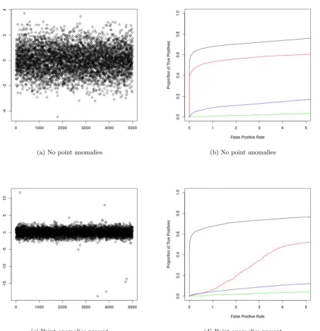
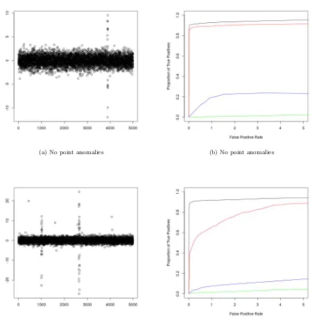
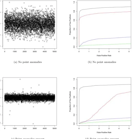
We obtained ROC curves for the four methods. For BreakoutDetection and PELT, we considered detected changes within 20 time points of true changes to be true positives and classified all other detected changes as false positives. For luminol and CAPA, we considered detected starting and end points of epidemic changes to be true positives if they were within 20 observations of a starting and end point respectively. The results regarding the precision of true positives in Section 5.2 suggest that the results in this section are robust with regard to the choice of error tolerance. We set the minimum segment length to ten for PELT, CAPA, and BreakoutDetection. To obtain the ROC curves we varied the penalty for epidemic segments in CAPA, the penalty in PELT, the threshold in luminol, and the beta parameter of BreakoutDetection.
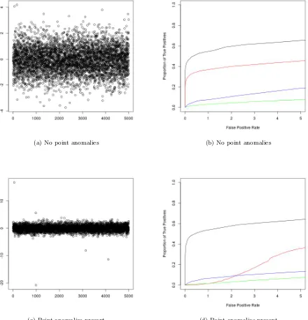
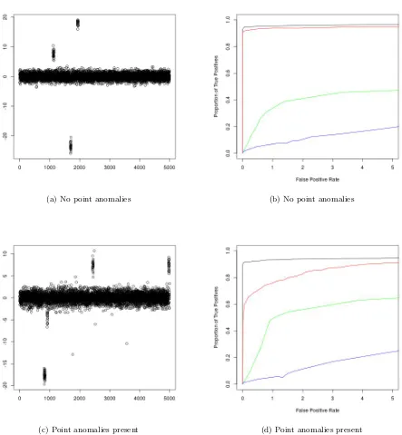
The resulting ROC curves, as well as examples of realisations of the data for the scenario of weak and strong changes in mean can be found in Figures 2 and 3 respectively. The results for joint changes in mean and variance, as well as changes in variance can be found in the supplementary material. We see that CAPA generally outperforms PELT, even in the absence of point anomalies. This is due to it having more statistical power, by exploiting the epidemic nature of the change. This becomes particularly apparent when the changes are weak. CAPA also outperform BreakoutDetection and luminol for epidemic changes in mean, the scenario for which these methods were developed. Moreover, the performance of CAPA is barely affected by the presence of point anomalies, unlike that of the non-robust methods. This observation remained true when we repeated our analysis withN(0,10002) distributed point anomalies. The ROC curves for these additional simulations can be
found in the supplementary material.
5.2
Precision
(a) No point anomalies (b) No point anomalies
[image:8.595.81.521.176.634.2](c) Point anomalies present (d) Point anomalies present
(a) No point anomalies (b) No point anomalies
[image:9.595.78.521.161.640.2](c) Point anomalies present (d) Point anomalies present
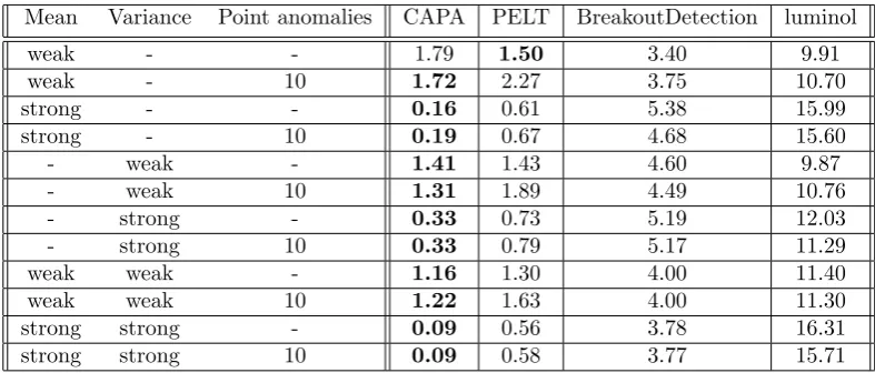
Mean Variance Point anomalies CAPA PELT BreakoutDetection luminol
weak - - 1.79 1.50 3.40 9.91
weak - 10 1.72 2.27 3.75 10.70
strong - - 0.16 0.61 5.38 15.99
strong - 10 0.19 0.67 4.68 15.60
- weak - 1.41 1.43 4.60 9.87
- weak 10 1.31 1.89 4.49 10.76
- strong - 0.33 0.73 5.19 12.03
- strong 10 0.33 0.79 5.17 11.29
weak weak - 1.16 1.30 4.00 11.40
weak weak 10 1.22 1.63 4.00 11.30
strong strong - 0.09 0.56 3.78 16.31
[image:10.595.100.494.52.220.2]strong strong 10 0.09 0.58 3.77 15.71
Figure 4: Precision of true positives measured in mean absolute distance for CAPA, PELT, luminol, and Break-outDetection
(a) With epidemic changes (b) Stationary data
Figure 5: Runtime of CAPA (black), PELT (red), BreakoutDetection (green), and luminol (blue)
the nearest estimated change across all the 12 scenarios. We used the default penalties for all methods (i.e. the default threshold for luminol and the BIC for PELT and CAPA) except BreakoutDetection, where we found that the default penalty returned no true positives at all for many scenarios. We therefore used the results we obtained when deriving the ROC curves to set the beta parameter to an appropriate level for each case.
The results of this analysis can be found in Figure 4. We see that CAPA is generally the most precise one. Moreover, its precision is not too strongly affected by the presence of point anomalies, unlike that of PELT, whose performance is significantly deteriorated by anomalies, especially when the signal is weak. The reason for this is that PELT fits additional changes in the presence of anomalies, which results in shorter segments. This leads to less accurate parameter estimates, which results in poorer estimates for the location of the changepoint. CAPA does not face this problem since the parameter of the typical distribution is shared across all segments. This remains true when the point anomalies are are a lot stronger, as can be seen in the supplementary material.
5.3
Runtime
[image:10.595.74.520.291.514.2]Figure 5 displays the average speed over 50 repetitions for the two cases. When comparing the slopes between 10000 and 50000 datapoints we note that it is very close to 2 for BreakoutDetection in both cases as well as CAPA and PELT for stationary data, suggesting quadratic scaling. In the presence of epidemic changes however, that slope is 1.26 for CAPA – 1.14 even between 25000 and 50000 datapoints – thus suggesting near linear runtime.
6
Application to Kepler Light Curve Data
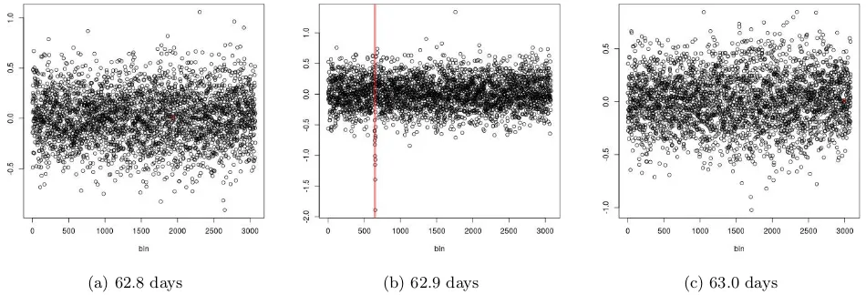
[image:11.595.61.536.175.337.2](a) 62.8 days (b) 62.9 days (c) 63.0 days
Figure 6: CAPA applied to the light curve of Kepler 1132 preprocessed using different periods.
We now apply CAPA to the Kepler light curve data, with the aim of detecting exoplanets via the so called transit method ([30]). As described in Section 1, this approach consists of repeatedly measuring a star’s brightness for a certain period of time, thus obtaining a so called light curve. Periodically recurring dips in the measurements then point towards the transit of a planet causing a small eclipse. Since the signal of transiting planets is known to be weak, we amplify it by exploiting its periodic nature. If the period of an orbiting planet were known, the signal of its transit could be strengthened by considering all data points to have been gathered at their measurement time modulo that period. We would thus obtain an irregularly sampled time series which we can transform into a regularly sampled time series by binning the data into equally sized bins of length approximately equal to the measurement interval of the Kepler telescope and taking the average within each bin. We could then apply CAPA to this preprocessed data, which would exhibit a stronger signal for any planet with the associated period. Detecting the signal for such a planet involves detecting a collective anomaly with a reduced mean. However we need to do this whilst being robust to the point anomalies in the data, and the potentially other collective anomalies associated with planets with different periods. The results obtained by applying this method, using the default penalties of our software implementation of CAPA, to the light curve of Kepler 1132 using a period of 62.8, 62.9, and 63.0 days can be found in Figure 6. We note that using a period of 62.9 days results in a promising dip, which is not present when using 62.8 or 63 days as period.
Given a light curve, the periods of exoplanets orbiting the corresponding star (if any are present) are obviously not known a priori. We can, however, apply the above approach for a range of periods, given the fact that the cost of running CAPA is comparable to that of binning the data. Since transits appear as periods of reduced mean, we record the strength of the strongest change in mean as defined by maxk(4µ,k) and estimated using
the sample mean and variance in the collective anomalies, and the estimated means and variance of the typical distribution. We expect this quantity to be largest for the periods of exoplanets. We identified the strength of the strongest change in mean for all periods from 1 day to 200 days with increments of 0.01 days for the light curve of Kepler 1132. The result of this analysis can be found in Figure 7. Note that the largest change in mean is recorded at a period of 62.89 days. As with spectral methods, we also observe resonance of the main signal at integer fractions of that period. This result is consistent with the existing literature, which considers Kepler 1132 to be orbited approximately every 62.892 days by the exoplanet Kepler 1132-b whose radius is about 2.5 times that of the earth ([20]).
Figure 7: The strongest change in mean, as measured by maxk(4µ,k), detected by CAPA for the lightcurve of
Kepler 1132. All periods from 1 to 200 days at 0.01 day increment were examined
7
Acknowledgements
This research has made use of the NASA Exoplanet Archive, which is operated by the California Institute of Technology, under contract with the National Aeronautics and Space Administration under the Exoplanet Exploration Program. The authors would like to thank the Isaac Newton Institute for Mathematical Sciences for support and hospitality during the programme Statistical Scalability when work on this paper was undertaken. This work was supported by EPSRC grant numbers EP/K032208/1 (INI), EP/R014604/1 (INI), EP/N031938/1 (StatScale), and EP/L015692/1 (STOR-i). The authors also acknowledge British Telecommunications plc (BT) for financial support and David Yearling and Kjeld Jensen in BT Research & Innovation for discussions.
8
Appendix: Proofs
This Appendix contains proofs for all the results in this papers. Proofs for Lemmata we use can be found in the supplementary material.
8.1
Proof of Proposition 1
Letm0≥m+ ˆl. We have
C(m) +
m0
X
t=m+1
C(xt,θˆ(m+1):m0) +β ≤C(k) +
m
X
t=k
C(xt,θˆ(k+1):m) + m0
X
t=m+1
C(xt,θˆ(m+1):m0) +β
≤C(k) +
m0
X
t=k+1
C(xt,θˆ(k+1):m0) +β,
8.2
Proof of Theorem 1
Before proving this theorem, we introduce some notation. We define the cost of a segment xi:j under the true
partition{0, t1, ..., tK, n} and true parameters to be
C(xi:j) = j
X
t=i
log(σ(t)2) +
j
X
t=i
η2t.
Note that this cost is additive, i.e. fora < b−1< b+ 1< cwe haveC(xa:c) =C(xa:b) +C(x(b+1):c), whilst the
fitted cost satisfies the inequality ˜C(xa:c)≥C˜(xa:b) + ˜C(x(b+1):c).
We also define the residual sum of squares Yi:j =P j
k=i(ηk−η¯i:j)2. Finally, we will work on the event sets
E1,E2,E3, E4,E5, andE6 which we define below using notationa:=a(i, j) =j−i+ 1
E1:=
aη¯i2:j<4(1 +) log(n), 1≤i≤j≤n ,
E2:=
n
Yi:j ≤a−1 + 2
p
(a−1)(2 +) log(n) + (4 + 2) log(n), 1≤i≤j≤no,
E3:={Yi:j≥c(a, n)(a−1), 1≤i < j≤n},
E4:=
( Ptk+1
t=tk−1(xt−x¯(tk−1):(tk+1))
2
σk2/3σk4/−31
> n−,
Ptk+2
t=tk(xt−x¯tk:(tk+2))
2
σk4/3σ2k/−31
> n−, 1≤k≤K−1 )
,
E5:= (x
tk−xtk+1)
2 σkσk−1
> n−, 1≤k≤K
,
E6:=
n
Yi:j ≥a−1−2
p
(a−1)(2 +) log(n), 1≤i≤j≤no,
wherec(a, n)<1 satisfies
a
2·
c(a, n)−1−log(c(a, n))
2 = (2 +) log(n).
Note thatc(a, n) is guaranteed to exits by the intermediate value theorem. Indeed, the functionf(x) =x−1−
log(x) is continuous and satisfies f(1) = 0 and f(x) → ∞ as x → 0+. The motivation for these events is as
follows: E1bounds the error in the estimates of the mean, whileE2,E3, andE6bound the error in the estimates of the variance. E5andE4 are needed to prevent the existence of segments length two and three respectively in which the observations lie to close to each other, which would encourage the algorithm to erroneously fit them in a short segment of low variance. We writeE=∩Ei.
We are now in a position to prove the following lemmata:
Lemma 1 (Yao 1988) P(E1)>1−K1n˜ −, for some constant K1˜ .
Lemma 2 P(E2)>1−K2n˜ −,P(E3)>1−K3n˜ −,P(E4)>1−K4n˜ −,P(E5)>1−K5n˜ −,P(E6)>1−K6n˜ −, andP(E7)>1−K7n˜ −for some constantsK2˜ ,K3˜ ,K4˜ ,K5˜ ,K6˜ , andK7˜ .
Lemma 3 There exists a constant C˜1 such thatYi:j−a−alog(Yi:j/a)≤C˜1log(n) holds onE for all 1≤i < j≤n.
Lemma 4 Let i, j be such that there exists somek such thattk−1< i < j ≤tk. The following holds given E :
0≤ C(xi:j)−C˜(xi:j)≤C2˜ log(n).
Lemma 5 Let i, j be such that ∃k such that tk−1 =i < j ≤tk or tk−1 < i < j =tk+ 1. The following then
holds givenE
C(xi:j)−C˜(xi:j)≤C3˜ log(n)
Lemma 6 Let a, b, c∈τ for some partitionτ ofxi,j such that ∃k such thattk−1< a < b < c≤tk. Then,
˜
C(xi:j, τ, β)−C˜(xi:j, τ−b, β)≥
3
4βlog(n)
1+δ,
whereτ−b=τ\ {b} holds on E for large enough n.
Lemma 7 For all α >0, there exists a constant κ˜(4k, α, δ, )decreasing in 4k such that C˜(xi:j)−(C(xi:tk) +
C x(tk+1):j
)≥αlog(n)1+δ holds on E ifj−t
k=tk+ 1−i≥˜κ(4k, α, δ, ) log(n)1+δ andj≤tk+1, i > tk−1for
We now define ˜κk = 2˜κ(4k,3β, δ, ), noting it decreases in4k, and the set of partitions
B:=
{0, t01, t02, ..., t0K, n} | |t0k−tk| ≤κ˜klog(n)1+δ 1≤k≤K ,
which are within ˜κklog(n)1+δ of the true partition.
We will show that, for large enough n, the optimal partition lies in B given the event set E. Given the probability ofE, this proves Theorem 1. Our approach will consist of showing that the cost of a partitionτ /∈ B
is higher than that of the true partition with the true parameters (see Proposition 4). We will achieve this by adding free changes to τ thus splitting up the series into multiple sub-segments each containing a single true changepoint and ˜κklog(n)1+δ points either side of it. This also defines a projection of τ onto the partitions of
the sub-segments. We define the set of partitions
Bk:=
{i−1, t0k, j} | |t0k−tk| ≤κ˜klog(n)1+δ
for segmentsxi:jfor which there exist aksuch that:tk−1+1≤i≤tk−κ˜klog(n)1+δ < tk+˜κklog(n)1+δ≤j≤tk+1
as an analogue ofB for the whole ofx.
Ifτ /∈ B, there must be at least one sub-segment for which the projection ofτ does not lie inBk. We will show
in Proposition 3, that the cost of the true partition using the true parameters is at leastO(log(n)1+δ) lower than
that of the projection ofτon such a segment. We will also show in Proposition 2 that the projections ofτ which are inBk have a cost which is at mostO(log(n)) lower than that of the true partition with true parameters.
Proposition 2 Let i, j ∈N, be such that there exists ak such that: tk−1+ 1≤i < tk < j≤tk+1, then there
exists a constantC˜4 such that given E,
C(xi:j) +βlog(n)1+δ−C˜(xi:j, τ, β)≤C4˜ log(n)
for all valid partitions τ of the form τ={i−1,ˆt, j}, if nis large enough.
Proof of Proposition 2: The following cases are possible:
Case 1: ˆt=tk. Then:
C(xi:j) +βlog(n)1+δ
−C˜(xi:j,{i−1,ˆt, j}, β) =C(xi:j)−
h ˜
C(xi:tk) + ˜C(x(tk+1):j)
i
≤2 ˜C2log(n),
where the inequality follows from Lemma 4.
Case 2: ˆt=tk+ 1. Then:
C(xi:j) +βlog(n)1+δ−C˜(xi:j,{i−1,ˆt, j}, β)
=C(xi:j)−
h ˜
C(xi:(tk+1)) + ˜C(x(tk+2):j)
i
≤( ˜C2+ ˜C3) log(n),
where the inequality follows from Lemmata 4 and 5.
Case 3: ˆt > tk+ 1. Then:
C(xi:j) +βlog(n)1+δ
−C˜(xi:j,{i−1,ˆt, j})≤ C(xi:j) + 2βlog(n)1+δ−C˜(xi:j,{i−1, tk,ˆt, j}, β)
=C(xi:j)−
h ˜
C(xi:tk) + ˜C(x(tk+1):ˆt) + ˜C(x(ˆt+1):j)
i
≤3 ˜C2log(n),
where the first inequality follows from the fact that introducing an unpenalised changepoint reduces cost and the second is a consequence of Lemma 4.
Case 4: ˆt=tk−1. Symmetrical to case 2.
Case 5: ˆt < tk−1. Symmetrical to case 3.
This finishes our proof.
Proposition 3 There exists a constant n4(β, δ, ), such that ∀i, j for which ∃k such that tk−1+ 1 ≤i≤ tk−
˜
κklog(n)1+δ < tk+ ˜κklog(n)1+δ ≤j≤tk+1
˜
C(xi:j, τ, β)−
C(xi:j) +βlog(n)1+δ
≥1
3βlog(n)
1+δ
holds for allτ /∈ Bk givenE andn > n4(β, δ, ).
Proof of Proposition 3: Consider τ0 ∈ B/ k. We consider the following three cases and denote H :=
d1
2κ˜klog(n)
Case 1: |τ0|= 2. We haveτ0 ={i−1, j}. Hence:
˜
C(xi:j, τ0, β)≥C˜(xi:(tk−H)) + ˜C(x(tk−H+1):(tk+H)) + ˜C(x(tk+H+1):j)
≥C˜(xi:(tk−H)) +C(x(tk−H+1):(tk+H)) + 3βlog(n)
1+δ+ ˜C(x
(tk+H+1):j)
≥2βlog(n)1+δ−2 ˜C2log(n) +
C(xi:j) +βlog(n)1+δ
,
where the second inequality follows from the definition ofH and Lemma 7 and the third from Lemma 4.
Case 2: |τ0|= 3. We haveτ0={i−1, tk+L, j}, where|L|>˜κklog(n)1+δ. We assumeL >0, the other case
being very similar. We have:
˜
C(xi:j,{i−1, tk+L, j}, β) = ˜C(xi:(tk+L)) + ˜C(x(tk+L+1):j) +βlog(n)
1+δ
≥C˜(xi:(tk−H−1)) + ˜C(x(tk−H):(tk+H)) + ˜C(x(tk+H+1):(tk+L))−
˜
C2log(n) +C(x(tk+L+1):j) +βlog(n)
1+δ
≥3βlog(n)1+δ−3 ˜C2log(n) +
C(xi:j) +βlog(n)1+δ
,
where the inequalities follow from of the definition ofH as well as Lemmata 7 and 4.
Case 3: |τ0| ≥ 4. Let τ0 = {a1, a2, ..., a|τ0|}, where a1 = i−1 and a|τ0| = j. There must exist a l ∈
{2, ...,|τ0| −1}, such thatal−1< tk andal+1> tk+ 1. We thus have:
˜
C(xi:j, τ0, β) = (|τ0| −3)βlog(n)1+δ+
l−2
X
m=1
+ |τ0|−1
X
m=l+1
h
˜
C(xam+1,am+1)
i
+ ˜C(x(al−1+1):al+1,{al−1, al, al+1}, β)
≥(|τ0| −2)βlog(n)1+δ+
l−2
X
m=1
+ |τ0|−1
X
m=l+1
C(xam+1,am+1)
+C(x(al−1+1):al+1)−(|τ
0| −3) ˜C2log(n)−C4˜ log(n)
=C(xi:j, τ, β) +βlog(n)1+δ+ (|τ0| −3)βlog(n)1+δ−
h
(|τ0| −3) ˜C2+ ˜C4ilog(n),
by Lemma 4 and Proposition 2. This finishes the proof.
Proposition 4 There exists a constantn5˜ (β, δ,4,˜δ, )decreasing in4 such that givenE, we have
˜
C(x1:n, τ, β)−
C(x1,n) +Kβlog(n)1+δ
≥1
4βlog(n)
1+δ
for allτ /∈ Bif n≥n˜5(β, δ,4,δ, ˜ ).
Proof of Proposition 4: First, consider the special case K= 0. For this case, τ /∈ B implies that ˆK≥1. We have
˜
C(x1:n, τ, β)≥C˜(x1:n,{0, n}, β) + ˆK
3
4βlog(n)
1+δ
≥ C(x1:n) + ˆK
3
4βlog(n)
1+δ
−C2˜ log(n),
where the first inequality follows from Lemma 6 and the second from Lemma 4.
Next assume K ≥ 1. Let τ /∈ B. We now introduce free changepoints l0, l1, ..., lK to break up the series
into multiple sub-series with one true changepoint each. We impose l0 = 0, lK =n, |lk−tk| >4˜κklog(n)1+δ
for 0 < k ≤ K and |lk −tk+1| > 4˜κklog(n)1+δ for 0 ≤ k < K. We also require that τ ∪ {l0, ..., lK} is a
valid partition (i.e. one which has segments of length at least two) and that there exists a ˆk such that τˆk :=
τ∩ {lˆk−1+ 1, lkˆ−1+ 2, ..., lkˆ}∈ B/ ˆk. We are guaranteed to find such pointsl0, l1, ..., lK ifnis such that
log(n)1+δ+˜δ≥12˜κklog(n)1+δ,
which is satisfied ifn >n5˜ (β, δ,4,δ, ˜ ), where ˜n5(β, δ,4,˜δ, ) decreases inδ. Indeed, we can choose points near the middle of the true segments which are not inτ, or by select points in τ if the former is impossible because there are too many point inτ near the middle of some segment.
Since introducing free changes reduces the cost we then have
˜
C(x1:n, τ, β)≥ K
X
k=1
˜
C(x(lk−1+1):lk, τk, β) = ˜C(x(lˆk−1+1):lkˆ, τˆk, β) +
X
k6=ˆk
˜
C(x(lk−1+1):lk, τk, β)
≥ C(x1:n, τ, β) +
1
3βlog(n)
1+δ−(K−1) ˜C4log(n),
where the second inequality follows from Propositions 2 and 3. This finishes the proof.
8.3
Proof of Theorem 2
In order to prove this result, we will use the following notation in this section: We define ˜CE(x1:n, τE, β, µ, σ) to
be the cost of an epidemic partitionτE ={ˆs1,e1, ...ˆ ˆsKˆ,eˆKˆ}under a penaltyβlog(n)1+δ and inferred parameters
of the typical distributionµ, σ. We defineCE(x1:n, β, µ, σ), to be the cost under the true partition using the true
parameters for the epidemic segments andµ, σ as estimates for the parameters of the typical distribution. We also define the set of epidemic partitions
BE=
{ˆs1,eˆ1, ...,ˆsK,ˆeK} | |ˆek−ek|<˜κklog(n)1+δ,|sˆk−sk|<κ˜klog(n)1+δ
as an epidemic equivalent ofB. Finally, we note that we can extend the definition of the event setE to epidemic changepoints by treating thesk andek like classical changepoints.
We will begin by proving a simplified version of the theorem in which we run our epidemic changepoint detection algorithm without allowing for epidemic changes of length one in variance only and imposing that each segment of the data allocated to the typical distribution is of length at least two. The reason for this is that this allows us to define an equivalent non-epidemic partition, whose segments must be of length at least two, for each epidemic partition. We also begin by assuming that the parameter of the typical distribution is known.
This simplified version captures the main ideas of the full proof. We will proceed to showing that the result also holds when the typical mean and variance are unknown. This will be followed by a proof of the full result by means of introducing and proving the consistency of a modified version of the classical changepoint detection algorithm described in the previous section which also allows for segments of length one.
For now, we assume that all segments are of length at least two and that the true parameters µ0 andσ0 are known. This allows us to use the fact that the cost of the true epidemic partition using the true parameters is exactly the same as the cost of the corresponding true non-epidemic partition using the true parameters with twice the penalty. We can therefore prove the following proposition, as a corollary of Proposition 4.
Proposition 5 There exists a constantn6˜ (β, δ,4,˜δ, ), decreasing in 4 such that for allτE0 ∈ B/ E
˜
CE(x1:n, τE0 , β, µ0, σ0)− CE(x1:n, β, µ0, σ0)≥
1
5βlog(n)
1+δ/2
holds on E for large enough n >n6˜ (β, δ,4,˜δ, ).
Proof of Proposition 5: We note that
˜
CE(x1:n, τE0, β, µ0, σ0)≥C˜
x1:n, τE0 ∪ {0, n},
1 2β
+β
2
ˆ
K
X
k=2
I{sk=ek−1}log(n)1+δ,
because using fitted parameters instead ofµ0 andσ0 for segments allocated to the typical distribution underτE0
can only reduce the cost. Additionally, two epidemic changes correspond to three classical changepoints if their end and starting points coincide. Moreover,
CE(x1:n, β, µ0, σ0) =C(x1:n) +Kβlog(n)1+δ.
Therefore:
˜
CE(x1:n, τE0 , β, µ0, σ0)− CE(x1:n, β, µ0, σ0)
≥C˜
x1:n, τE0 ∪ {0, n},
1 2β
+β
2
ˆ
K
X
k=2
I{sk =ek−1}log(n)1+δ−
C(x1:n) + 2K
β
2log(n)
.
This leaves two possibilities. IfτE0 ∪ {0, n}∈ B/ then the above will exceed 1
4βlog(n)
1+δ,
by proposition 4. Since τE0 ∈ B/ E, the only way we can have τE0 ∪ {0, n} ∈ B is if there exists a k such that
sk =ek−1. In that case the difference will exceed
1
2βlog(n)
1+δ
−(2K+ 1) ˜C4log(n),
by Proposition 2. This finishes the proof.
We can now use this proposition to prove Theorem 2 in the same way we used 4 to prove Theorem 1.
Proof of Theorem 2: Proposition 5 proves Theorem 2 as Lemmata 1 and 2 imply thatP(E)≥1−( ˜K1+ ˜
K2+ ˜K3+ ˜K4+ ˜K5+ ˜K6)n−.
Lemma 8 There exists a constants K8˜ ,D1, andD2 such that for large enough n
P |µˆ−µ0| ≤D1σ0 r
log(n)
n , ˆ σ2 σ2 0 −1 ≤D2 r log(n)
n
!
≥1−K8n˜ −
We can use this Lemma above to introduce a new event E7 stating that the estimated parameters are close to the true parameters.
E7:= (
|µˆ−µ0| ≤D1σ0
r log(n)
n , ˆ σ2 σ2 0 −1 ≤D2 r log(n)
n
)
.
This event bounds the effect of using the estimated typical parameters instead of the true parameters for the cost of the true distribution with true non-typical parameters. Indeed, the following lemma holds:
Lemma 9 There exists a constantC7˜ such that given E andE7 and n large enough we have:
˜
CE(x1:n, β,µ,ˆ σˆ)− CE(x1:n, β, µ0, σ0)≤C˜7log(n).
We can use this lemma to prove the following extension of Proposition 5 to the case when the typical parameters are inferred.
Proposition 6 There exists a constantn˜7(β, δ,4,δ, ˜ )decreasing in4 such that for all τE0 ∈ B/ E
˜
CE(x1:n, τE0 , β,µ,ˆ σˆ)− CE(x1:n, β,µ,ˆ σˆ)≥
1
5βlog(n)
1+δ/2
holds on E∩E7 forn >n7˜ (β, δ,4,δ, ˜ ).
Proof of Proposition 6: We note that, as before,
˜
CE(x1:n, τE0, β,µ,ˆ ˆσ)≥C˜
x1:n, τE0 ∪ {0, n},
1 2β +β 2 ˆ K X k=2
I{sk=ek−1}log(n)1+δ
CE(x1:n, β, µ, σ) =C(x1:n) +Kβlog(n)1+δ,
Therefore we now have
˜
CE(x1:n, τE0, β,µ,ˆ σˆ)− CE(x1:n, β,µ,ˆ σˆ)
≥C˜
x1:n, τE0 ∪ {0, n},
1 2β +β 2 ˆ K X k=2
I{sk=ek−1}log(n)1+δ−
C(x1:n) + 2K
β
2 log(n)
1+δ
−C˜7log(n),
by applying Lemma 9. The rest of the proof is identical to that of Proposition 5, with an addedO(log(n)) term. In order to be able to extend Proposition 6 to the case in which we allow epidemic changes of length one in variance only, as well as segments of the typical distribution which are of length one, we will prove the consistency of the following adaptation of the algorithm detecting classical changepoints we introduced in the previous section. We now let the segment costs be
˜
C(xi:j) = ˜C(xi:j,{i−1, j}) =
(ˆtk+1−ˆtk) log
Ptkˆ+1 ˆ
tk+1(xt−x¯(ˆtk+1):ˆtk+1) 2
(ˆtk+1−ˆtk)
!
+ 1 !
i < j,
minnlog(˜σ2) +(xi−µ˜)2
˜
σ2 ,1 + log(γσ˜2+ (xt−µ˜)2)
o
i=j,
where|µ˜−µk0| ≤D1σk0
q
log(n)
n and|
˜
σ2 σ2
k0
−1|< D2
q
log(n)
n fork
0 either k−1,k, ork+ 1, whenibelongs to the
kth segment. Given E7 the range of allowed ˜σ2 and ˜µ is therefore guaranteed to contain the estimated typical
parameters ˆσ2 and ˆµ when applied to x. The algorithm can obviously not be implemented in practice, as it
requires knowledge of the true parameters. It is nevertheless a consistent method.
To prove this, we need to define a last event set E8 which controls the newly introduced segments of length
one:
E8:=
|xt−µk+1| ≥σkn−2+, |xt−µk−1| ≥σkn−2+, 1≤t≤n ,
We can prove the following probability bounds
We can now prove the following proposition, adapted from Proposition 4 for this modified penalised cost approach:
Proposition 7 There exists a constantn7˜ (β, δ,4,˜δ, )such that givenE∩E8, we have
˜
C(x1:n, τ, β)−
C(x1,n) +Kβlog(n)1+δ
≥1
5βlog(n)
1+δ
for allτ /∈B if n≥n˜7(β, δ,4,δ, ˜ )
Proof of Proposition 7: Identical to the proof of Proposition 4. We just need to replace Lemma 4 by
Lemma 11 There exists a constant C˜20 such that ifi, j are such that there exists somek such that tk−1 < i≤ j≤tk, then givenE∩E7 andn large enough
C(xi:j)−C˜(xi:j)≤C˜20log(n).
to also account for the newly added segments of length one. We can now prove that
Proposition 8 There exists a constantn8˜ (β, δ,4,˜δ, )decreasing in4 such that for all τE0 ∈ B/ E
˜
CE(x1:n, τE0 , β,µ,ˆ σˆ)− CE(x1:n, β,µ,ˆ σˆ)≥
1
5βlog(n)
1+δ/2
holds on E∩E7∩E8 forn >n8˜ (β, δ,4,˜δ, ).
holds even when we allow for epidemic changes of length one in variance only and do not impose that segments allocated to the typical distribution have to be of length at least two.
Proof of Proposition 8: Identical to the proof of Proposition 6 using Proposition 7 instead of Proposition 4.
Proof of Theorem 2: Proposition 8 proves Theorem 2 since Lemmata 1, 2, 8, and 10 show thatP(E∩E7∩
E8)≥1−( ˜K1+ ˜K2+ ˜K3+ ˜K4+ ˜K5+ ˜K6+ ˜K7+ ˜K8)n−.
References
[1] Aston, J. A. and Kirch, C. (2012) Evaluating stationarity via change-point alternatives with applications to fMRI data. The Annals of Applied Statistics,6, 1906–1948.
[2] Bardwell, L. and Fearnhead, P. (2017) Bayesian detection of abnormal segments in multiple time series. Bayesian Analysis,12, 193–218.
[3] Breunig, M., Kriegel, H.-P., Ng, R. T. and Sander, J. (2000) LOF: Identifying density-based local outliers. Proceedings of the 2000 ACM Sigmod International Conference on Management of Data, 93–104.
[4] Chandola, V., Banerjee, A. and Kumar, V. (2009) Anomaly detection: A survey. ACM computing surveys (CSUR),41, 15.
[5] Cleveland, R. B., Cleveland, W. S. and Terpenning, I. (1990) STL: A seasonal-trend decomposition procedure based on loess. Journal of Official Statistics,6, 3.
[6] Fearnhead, P. and Rigaill, G. (2017) Changepoint detection in the presence of outliers. Journal of the American Statistical Association.
[7] Fryzlewicz, P. (2014) Wild binary segmentation for multiple change-point detection.The Annals of Statistics,
42, 2243–2281.
[8] Guha, S., Mishra, N., Roy, G. and Schrijvers, O. (2016) Robust random cut forest based anomaly detection on streams. InInternational Conference on Machine Learning, 2712–2721.
[9] Hampel, F. R., Ronchetti, E. M., Rousseeuw, P. J. and Stahel, W. A. (1986)Robust Statistics - The Approach Based on Influence Functions. Wiley.
[10] Jackson, B., Scargle, J. D., Barnes, D., Arabhi, S., Alt, A., Gioumousis, P., Gwin, E., Sangtrakulcharoen, P., Tan, L. and Tsai, T. T. (2005) An algorithm for optimal partitioning of data on an interval.IEEE Signal Processing Letters, 12, 105–108.
[12] Jeng, X. J., Cai, T. T. and Li, H. (2012) Simultaneous discovery of rare and common segment variants. Biometrika,100, 157–172.
[13] Jureˇckov´a, J. and Picek, J. (2005) Robust statistical methods with R. CRC Press.
[14] Killick, R. and Eckley, I. (2014) changepoint: An R package for changepoint analysis. Journal of statistical software,58, 1–19.
[15] Killick, R., Fearnhead, P. and Eckley, I. A. (2012) Optimal detection of changepoints with a linear compu-tational cost. Journal of the American Statistical Association,107, 1590–1598.
[16] Laurent, B. and Massart, P. (2000) Adaptive estimation of a quadratic functional by model selection.Annals of Statistics, 1302–1338.
[17] Levin, B. and Kline, J. (1985) The cusum test of homogeneity with an application in spontaneous abortion epidemiology. Statistics in Medicine,4, 469–488.
[18] Ma, T. F. and Yau, C. Y. (2016) A pairwise likelihood-based approach for changepoint detection in multi-variate time series models. Biometrika,103, 409–421.
[19] Maheshwari, R., Yang, Y., Hou, R., Li, B. and Liang, Z. (2014) luminol: Anomaly detection and correlation library. URL:https://github.com/linkedin/luminol.
[20] Morton, T. D., Bryson, S. T., Coughlin, J. L., Rowe, J. F., Ravichandran, G., Petigura, E. A., Haas, M. R. and Batalha, N. M. (2016) False positive probabilities for all kepler objects of interest: 1284 newly validated planets and 428 likely false positives. The Astrophysical Journal,822, 86.
[21] Muler, N., Pena, D. and Yohai, V. J. (2009) Robust estimation for ARMA models. The Annals of Statistics,
37, 816–840.
[22] Muler, N. and Yohai, V. J. (2002) Robust estimates for ARCH processes. Journal of Time Series Analysis,
23, 341–375.
[23] — (2008) Robust estimates for GARCH models. Journal of Statistical Planning and Inference, 138, 2918– 2940.
[24] Mullally, S. E. (2016) Data validation time series file: Description of file format and content.
[25] Pimentel, M. A., Clifton, D. A., Clifton, L. and Tarassenko, L. (2014) A review of novelty detection. Signal Processing,99, 215–249.
[26] Reiss, R.-D. (2012)Approximate distributions of order statistics: with applications to nonparametric statis-tics. Springer science & business media.
[27] Robinson, L. F., Wager, T. D. and Lindquist, M. A. (2010) Change point estimation in multi-subject fMRI studies. Neuroimage,49, 1581–1592.
[28] Rousseeuw, P. and Yohai, V. J. (1984) Robust regression by means of S-estimators. InRobust and nonlinear time series analysis, 256–272. Springer.
[29] Rousseeuw, P. J. (1985) Multivariate estimation with high breakdown point. Mathematical statistics and applications, 8, 283–297.
[30] Sartoretti, P. and Schneider, J. (1999) On the detection of satellites of extrasolar planets with the method of transits. Astronomy and Astrophysics Supplement Series,134, 553–560.
[31] Siegmund, D., Yakir, B. and Zhang, N. R. (2011) Detecting simultaneous variant intervals in aligned se-quences. The Annals of Applied Statistics, 645–668.
[32] Smyth, P. (1994) Markov monitoring with unknown states. IEEE Journal on Selected Areas in Communi-cations,12, 1600–1612.
[33] Struve, O. (1952) Proposal for a project of high-precision stellar radial velocity work. The Observatory,72, 199–200.
[34] Yao, Q. (1993) Tests for change-points with epidemic alternatives. Biometrika,80, 179–191.
[35] Yao, Y.-C. (1988) Estimating the number of change-points via schwarz’ criterion. Statistics & Probability Letters, 6, 181–189.
9
Supplementary Material
9.1
Proofs of Lemmata
Lemma 1 (Yao 1988) P(E1)>1−K1n˜ −, for some constant K1˜ .
Proof of Lemma 1: See [35].
Lemma 2 P(E2)>1−K2n˜ −,P(E3)>1−K3n˜ −,P(E4)>1−K4n˜ −,P(E5)>1−K5n˜ −,P(E6)>1−K6n˜ −, andP(E7)>1−K7n˜ −for some constantsK2˜ ,K3˜ ,K4˜ ,K5˜ ,K6˜ , andK7˜ .
Proof of Lemma 2: We note that Yi:j∼χ2a−1. [16] proved that
P
−2√kx≤χ2k−k≤2√kx+ 2x≥1−2e−x.
Therefore:
P
−2p(a−1)(2 +) log(n)≤Yi:j−(a−1)≤2
p
(a−1)(2 +) log(n) + 2(2 +) log(n)≥1−2n−(2+).
A Bonferroni correction therefore givesP(E2∩E6)>1−2n−.
We can derive the following Chernoff bound fork≥1 and 0≤˜c <1:
P χ2k≤kc˜
=P expθ(χ2k−k˜c)
≥1≤E expθ(χ2k−k˜c)
=e−k˜cθE
eθχ2k
=e−k˜cθ
1
1−2θ
k/2
,
holds for allθ <0. Settingθ= 12(1−1 ˜
c) we thus get
P χ2k ≤k˜c
≤exp
−k
2(˜c−1−log(˜c))
.
Thus if we letc(a, n)<1 be such that
a
2·
c(a, n)−1−log(c(a, n))
2 = (2 +) log(n),
and writec:=c(a, n) for simplicity, we have
P(Yi:j≤c(a−1))≤exp
−a−1
2 (c−1−log(c))
≤exp−a
4(c−1−log(c))
=n−(2+),
fora≥2. A Bonferroni correction then givesP(E3)>1−n−. Next we note that
σkηtk+1+µk+1−µk−σkηtk
√
σk+1σk
∼N
µ
k+1−µk
√
σk+1σk
,σ 2
k+1+σ 2
k
σk+1σk
.
Consequently, we have that:
P
|σk+1ηtk+1+µk+1−µk−σkηtk|
√
σk+1σk
≤n−
≤
s
2σk+1σk
π(σ2
k+1+σk2−1) n−≤
r 1
πn
−.
A Bonferroni correction then givesP(E5)>1−K/√πn−.
Finally, we have:
xt−x¯tk:(tk+2)∼
N2µk−2µk+1 3 ,
4σk2+2σ2k+1
9
t=tk,
Nµk+1−µk
3 ,
2σk2+5σ2k+1
9
t=tk+ 1, tk+ 2,
which means that
(xt−x¯tk:(tk+2))
2≥4σ 2
k+ 2σ
2
k+1
9 n
−, t=t k,
(xt−x¯tk:(tk+2))
2≥1σ 2
k+ 5σ
2
k+1
9 n
−, t=t
holds with probability exceeding 1−3n−. Adding up the three inequalities then gives
tk+2
X
t=tk
(xt−x¯tk:(tk+2))
2≥12σ 2
k+1+ 6σ 2
k
9 n
−≥2σ4/3
k+1σ 2/3
k n
−.
By a similar argument,
tk+1
X
t=tk−1
(xt−x¯(tk−1):(tk+1))
2≥2σ2/3
k+1σ 4/3
k n
−
must also hold with probability 1−3n−. A Bonferroni correction then givesP(E4)≥1−6Kn−. This finishes our proof.
Lemma 3 There exists a constant C˜1 such thatYi:j−a−alog(Yi:j/a)≤C˜1log(n) holds onE for all 1≤i < j≤n.
Proof of Lemma 3: Consider the functionf(x) =x−a−alog(x/a). This function decreases monotonically on (0, a) and increases monotonically on (a,∞). SinceE2 andE3boundYi:j from above and below respectively
we only have to show thatYi:j−a−alog(Yi:j/a)≤C1˜ log(n) holds for the bounds in order to prove the lemma.
Part 1: Upper bound: ByE2there exist constantsM andM0such thatYi:j≤a+M
p
alog(n)+M0log(n). Substituting this upper bound forYi:j gives:
Yi:j−a−alog
Y
i:j
a
≤Mpalog(n) +M0log(n)−alog 1 + M p
alog(n) +M0log(n)
a
!
. (4)
Case 1: a≤log(n). In that case we can bound equation (4) by
Mpalog(n) +M0log(n)≤(M+M0) log(n).
Case 2: a≥log(n). We can use the fact that log(1 +x)≥x−x2, ∀x >0 to bound equation (4) by
(Mpalog(n) +M0log(n))2
a ≤(M+M
0)2log(n).
Part 2: Lower bound: E3implies thatYi:j≥c(a, n)(a−1). Substituting this bound gives
Yi:j−a−alog
Y
i:j
a
≤a(c(a, n)−1−log(c(a, n))−c−alog a−1
a
≤4(4 +) log(n) +alog
a
a−1
≤4(4 +) log(n) + a
a−1 ≤4(4 +) log(n) + 2.
This finishes the proof.
Lemma 4 Let i, j be such that there exists somek such thattk−1< i < j ≤tk. The following holds given E :
0≤ C(xi:j)−C˜(xi:j)≤C2˜ log(n).
Proof of Lemma 4: This lemma bounds the reduction in cost we can obtain by using a mean and variance fitted to a segment rather than the true mean and variance of the segment. The left bound follows from the fact
˜
C(xi:j) fits the mean and variance to minimise the log likelihood on the segment xi:j. The right bound follows
from Lemma 3 andE1. Indeed,
C(xi:j)−C˜(xi:j) = (j−i+ 1) log(σ2k) + j
X
t=i
η2t−(j−i+ 1)
log
σ2
kYi:j
j−i+ 1
+ 1
=aη¯i:j2+Yi:j−alog
Y
i:j
a
−a≤C˜1+ 4 +
log(n),
which finishes the proof.
Lemma 5 Let i, j be such that ∃k such that tk−1 =i < j ≤tk or tk−1 < i < j =tk+ 1. The following then
holds givenE
Proof of Lemma 5: This Lemma is very similar to Lemma 4, except that we slightly relax the constraint that all the data has to be located between two changepoints. This is needed because of the minimum segment length of two. We will prove this lemma for the case where tk−1 =i, the other case being very similar. We
consider 3 cases:
Case 1: j=tk−1+ 1. We have that:
C(xi:j)−C˜(xi:j) = log(σ2k) + log(σ
2
k−1) +η 2
tk−1+η 2
tk−1+1−2 log
(x
tk+1−xtk)
2
4
−2
≤(8 + 2) log(n)−2 log (x
tk+1−xtk)
2
4σk−1σk
−2≤(8 + 4) log(n) + 2 log(4)−2,
where the first inequality follows fromE1and the second from E5.
Case 2: j=tk−1+ 2. We have:
C(xi:j)−C˜(xi:j) = 2 log(σk2) + log(σ
2
k−1) +
tk−1+2
X
t=tk−1
ηt2−3 log
Ptk−1+2
t=tk−1(xt−x¯(tk−1):(tk−1+2)) 2
3
!
−3
≤2 log(σ2k) + log(σ2k−1) + (12 + 3) log(n)−3 log n −σ4/3
k σ
2/3
k−1
3
!
−3
= (12 + 6) log(n) + 3 log(3)−3,
where the inequality follows fromE1andE4.
Case 3: j > tk−1+ 2. We have:
C(xi:j)−C˜(xi:j)≤
h
C xi:(i+1)
−C˜ xi:(i+1)
i
+hC x(i+2):j
−C˜ x(i+2):j
i
≤(8 + 4) log(n) + 2 log(4)−2 + ˜C2log(n),
where the second inequality follows from case 1 and Lemma 4.
Lemma 6 Let a, b, c∈τ for some partitionτ ofxi,j such that ∃k such thattk−1< a < b < c≤tk. Then,
˜
C(xi:j, τ, β)−C˜(xi:j, τ−b, β)≥
3
4βlog(n)
1+δ,
whereτ−b=τ\ {b} holds on E for large enough n.
Proof of Lemma 6: This lemma applies Lemma 4 to show that removing false positives reduces the overall cost.
˜
C(xi:j, τ, β)−C˜(xi:j, τ−b, β) = ˜C x(a+1):b
+ ˜C x(b+1):c
−C˜ x(a+1):c
+βlog(n)1+δ
≥ C x(a+1):b
+C x(b+1):c
− C x(a+1):c
+βlog(n)1+δ−2 ˜C2log(n)≥
3
4βlog(n)
1+δ,
for large enoughn.
Lemma 7 For all α >0, there exists a constant κ˜(4k, α, δ, )decreasing in 4k such that C˜(xi:j)−(C(xi:tk) +
C x(tk+1):j
)≥αlog(n)1+δ holds on E ifj−t
k=tk+ 1−i≥˜κ(4k, α, δ, ) log(n)1+δ andj≤tk+1, i > tk−1for
alln >2.
Proof of Lemma 7: This lemma shows that not having an estimated changepoint near a true changepoint leads to high costs. Letj−tk=tk+ 1−i=D. We have:
1 2D
j
X
t=i
(xt−x¯i:j)2=
σ2
kYi:tk+σ
2
k+1Y(tk+1):j
2D +
1
4 µk+σkη¯i:tk−µk+1−σk+1η¯(tk+1):j
2
.
NowE2 implies that
σk2Yi:tk+σ
2
k+1Y(tk+1):j
2D ≥
σk2+σk2+1
2D
D−1−2p(D−1)(2 +) log(n)
=σkσk+1 1 +
42
σ,k
2 !
1− 1
D −2
r
(2 +) log(n)
D
!