BIROn - Birkbeck Institutional Research Online
Barros, Joana and Feitosa, F. (2018) Uneven geographies: exploring the
sensitivity of spatial indices of residential segregation.
Environment and
Planning B: Urban Analytics and City Science 45 (6), pp. 1073-1089. ISSN
2399-8083.
Downloaded from:
Usage Guidelines:
Please refer to usage guidelines at or alternatively
Uneven geographies: exploring the sensitivity of spatial
indices of residential segregation
Joana Barros
1, Flavia F. Feitosa
21Department of Geography, Birkbeck, University of London, UK. Malet Street, London WC1E 7HX, UK. E-mail: [email protected]
2Federal University of ABC (UFABC), Center for Engineering, Modeling and Applied Social Sciences, Alameda da Universidade, Anchieta, São Bernardo do Campo, SP, Brazil. E-mail: [email protected]
Abstract
There has been extensive use of segregation indices for measuring residential segregation since the 1950s, with continuous progress made in the field. Recent developments include the propositions of spatial global and local versions of traditionally used segregation indices, which have opened avenues for representing and analysing segregation as a multiscale and spatially-varying phenomenon. Much less explored has been the issue of how important research design choices, such as the extent of geographical boundaries, grouping systems and scales of analysis, can influence the measurement of segregation. This paper contributes in this direction by investigating the impact of such decisions in the outcomes of the indices of generalized dissimilarity (D) and information theory (H) using a set of sensitivity analysis. Using a comparative study between London and São Paulo as basis, results obtained with different geographical boundaries, grouping systems and scales for the two indices are analysed visually and quantitatively. Results suggest that although D and H depict the same spatial dimension of segregation (unevenness/clustering), they present different sensitivity to geographical boundaries and grouping systems. The study also revealed how the two indices unfold different aspects of the segregation, which impact on their interpretation and applicability. The study concludes with a discussion of the considerations on research design choices concerning the interpretation of the results, which indicate the two indices should not be used interchangeably.
Keywords
segregation, generalized dissimilarity index, information theory index, sensitivity analysis.
1. Introduction
However, spatial segregation is not desirable for two main reasons. The first is it decreases the opportunities of intergroup interaction which tends to decrease the integration amongst different groups in the urban society. The second is that different groups tend to have unequal access to urban resources and facilities which is dictated by their residential location. The issues with spatial segregation become clearer when focus is given to minority and/or socially disadvantaged groups as in most segregation studies, which traditionally look into ethno-racial minorities or socio-economic disadvantaged groups.
Segregation indices have been extensively used for measuring segregation since the 1950s. Measures of unevenness have been widely used to depict residential segregation thanks to the popularity of the dissimilarity index (Duncan and Duncan, 1955) and its generalized (multi-group) version (Sakoda, 1981). In fact, the extent of the use of dissimilarity index in particular was such that despite shortcomings of the metric (and preference to other indices), its continued use was recommended so the comparability with the existing body of literature would be maintained (Massey and Denton, 1988).
The suitability of segregation indices for empirical studies as well as their ability to provide reliable comparability between case studies, however, have been questioned. This was mainly due to the dependence of segregation indices on overall system variables such as absolute and relative size of population groups, which deemed the use of thresholds across case studies as well as across time periods of the same study area as unreliable (Johnston et al., 2007; Poulsen et al., 2002). Other reported issues also affect the confidence in results, such as when units of analysis are very small areas (i.e. census tracts) and/or contain very low population counts on minority groups (Voas and Williamson, 2000).
Segregation indices have also been widely criticised due to their global nature, where a single figure is used to represent an entire geographical area, ignoring spatial variation in segregation across geographical areas. In addition, it was recognised that traditional indices are insensitive to the spatial arrangement of population among areal units – an issue that became known as the checkerboard problem (White, 1983). These problems were addressed by the development of spatial and local indices (Feitosa et al., 2007; O’Sullivan and Wong, 2007; Reardon and O’Sullivan, 2004; Wong, 2003).
Segregation studies have also recognized that different segregation indices should be used in order to capture the different dimensions of the phenomenon (Massey and Denton, 1988; Reardon and O’Sullivan, 2004). Reardon and O’Sullivan (2004) proposed these dimensions are organised as two axis of spatial segregation: one axis ranging from evenness to clustering and another ranging from isolation to exposure. The dimension evenness/clustering concerns the balance of the spatial distribution of population groups and the isolation/exposure refers to the chance of having members from different groups (or same group, in the case of isolation) living in the same neighbourhood.
(2004) appointing the information theory index (Theil and Finizza, 1971) as the most reliable one, the dissimilarity index remains a popular choice. As studies usually adopt one or the other, there has not been much discussion on the implications of this choice on the outcomes of analysis and both indices remain used interchangeably, in both aspatial and spatial versions.
The recent developments in segregation measurement, such as global and local spatial indices, have opened new avenues for exploring residential segregation. While it is now possible to explore spatial patterns and understand how segregation varies in space (Catney, 2017; Lloyd and Shuttleworth, 2012) as well as investigate the multiscalar nature of segregation (Catney, 2017; Clark et al., 2015; Fowler, 2016; Östh et al., 2015; Reardon et al., 2008), the relationship between global measures and their local variation across scales has received little, if any, attention.
This study aims to contribute to a better understanding of the spatial segregation indices and their application to empirical studies by applying spatial global and local versions of two popular evenness/clustering indices, generalized dissimilarity (D) and information theory (H), to two case studies: São Paulo and London metropolitan areas. More specifically, the study looks at the effect of essential segregation measurement research design choices, such as the delimitation of geographical areas, grouping systems and scales of analysis, on the outcomes of the two indices. Using a set of sensitivity analysis, measurements obtained from experiments designed with different settings using both indices are compared, and their differences quantified using correlation analysis. Both global and local spatial indices are calculated for all experiments and the nuances revealed by local analyses in comparison to global measurements are explored.
The study is the by-product of a larger research project which looks into the relationship between spatial segregation and transport accessibility in the two equally large but very distinct metropolitan regions. São Paulo and London were selected for both their similarities and differences. Both municipalities present comparable population and area and both regions have a strong CBD and central denser areas. Both regions also present distinctive and divisive spatial segregation of income, social and ethnic group which were worth investigating. They also present striking differences which challenge their comparability using segregation indices, including size, nature of urban development, composition of population and their distribution in space. While these two particular case studies present significant comparative challenges, their study also presents an opportunity for showcasing the application of the same methodology to different areas in a comparative fashion.
highlighting issues and considerations for the effective use of both D and H in empirical studies.
2. Spatial Indices of Segregation
The approach adopted in this study follows that of Feitosa et al. (2007) to compute global and local spatial versions of D and extends it to H. It assumes an urban area has different localities, i.e., places where people live and exchange experiences, and represents the core of such localities by the centroid of areal units (e.g. census tracts). However, the population characteristics of a locality j are not restricted to the limits of areal unit j. Instead, they are expressed by its local population intensity, which is a geographically-weighted average of population data. The local population intensity of locality j (𝐿̆𝑗) and the local population of group m in the locality j (𝐿̆𝑗𝑚) are computed
using a kernel estimator placed on the centroid of areal unit j and the weights are given by the choice of a distance decay function and a bandwidth parameter (Feitosa et al., 2007):
𝐿̆𝑗 = ∑ 𝑘
𝐽
𝑗=1
(𝑁𝑗) (1)
and
𝐿̆𝑗𝑚 = ∑ 𝑘
𝐽
𝑗=1
(𝑁𝑗𝑚). (2)
, where J is the total number of areal units in the study area; 𝑁𝑗 and 𝑁𝑗𝑚 are,
respectively, the total population and the total population of group m in areal unit j; and k is the kernel estimator which estimates the influence of each areal unit on the locality j (normalized weight). Based on 𝐿̆𝑗 and 𝐿̆𝑗𝑚, the local proportion of group m
in locality j (𝜏̆𝑗𝑚 ) can be computed as:
𝜏̆𝑗𝑚 = 𝐿̆𝑗𝑚 𝐿̆𝑗
(3)
All global and local spatial indices used in this study, summarized in Table 1, require the calculation of local population intensities for all the localities of the study area. While global indices summarize the segregation degree of the entire study area, local indices are obtained by decomposing global indices, demonstrating how much each locality contributes to global indices and allowing segregation to be depicted as a spatially variant phenomenon.
Table 1 - Global and local spatial segregation indices
GLOBAL SPATIAL INDICES
Spatial generalized dissimilarity
𝐷̆ = ∑ ∑2𝑁𝐼𝑁𝑗
𝑀
𝑚=1 𝐽
𝑗=1
|𝜏̆𝑗𝑚− 𝜏𝑚|
where
(4)
index 𝐷̆
𝐼 = ∑ (𝜏𝑚)(1 − 𝜏𝑚) 𝑀
𝑚=1
(5) from 0 to 1, where 0 stands for the minimum degree of evenness and 1 for the maximum degree.
Spatial information theory index
𝐻̆
𝐻̆ = ∑ [𝑁𝑗(𝐸 − 𝐸̆𝐸𝑁 𝑗)]
𝐽
𝑗=1
where
(6) The global index Theil’s entropy index, a measure 𝐻̆ relies on of diversity, to compare the entropy of the whole study area (E) with the entropy of localities (𝐸̆𝑗). It captures the average of the
entropy of the localities and expresses it as a fraction of the entropy of the whole study area. It varies between 0, in which all localities have the same entropy of the study area (maximum
integration), and 1, in which all localities contain only one group (maximum segregation).
𝐸 = ∑ (𝜏𝑚)ln (𝜏1 𝑚) 𝑀
𝑚=1
(7)
𝐸̆𝑗 = ∑ (𝜏̆𝑗𝑚)ln (𝜏̆1 𝑗𝑚) 𝑀
𝑚=1
(8)
LOCAL SPATIAL INDICES
Spatial generalized dissimilarity index 𝑑̆𝑗
𝑑̆𝑗 = ∑
𝑁𝑗
2𝑁𝐼
𝑀
𝑚=1
|𝜏̆𝑗𝑚− 𝜏𝑚|
(9) The local index 𝑑̆𝑗 presents only
positive values and indicates how much each locality contributes to the global index 𝐷̆.
Spatial information theory index
ℎ̆𝑗
𝒉̆𝒋=
𝑵𝒋(𝑬 − 𝑬̆𝒋)
𝑬𝑵 (10)
The local index ℎ̆𝑗 presents
negative values when the locality j
has its local entropy 𝐸̆𝑗 greater
than the global entropy 𝐸 (local is more diverse than the whole) and positive values when the opposite happens.
Notation: J : total number of areal units in the study area
M : total number of population groups
N : total population in the study area
𝑁𝑚 : population of group m in the study area
Nj : total population in areal unit j
𝑁𝑗𝑚 : population of group m in areal unit j
𝐿̆𝑗 : local population intensity in locality j
𝐿̆𝑗𝑚 : local population of group m in the locality j
𝜏𝑚 : proportion of group m in the study area
𝜏̆𝑗𝑚 : local proportion of group m in locality j
3 Research design options for segregation studies
research design choices such as scales of analysis, delimitation of geographical boundaries of study areas and variations in grouping systems have not yet been systematically tested.
Below each of these design options is discussed and the choices made for each of the two study areas detailed. Due to their differences, the comparative study between São Paulo and London metropolitan regions requires a number of compromises and design choices which make the study suitable as a test bed to showcase nuances in the outcomes of segregation indices applied to empirical studies. While the design choices presented here have been made with the purpose of illustrating the challenges imposed by those choices, they have all been made on an empirical basis and are applicable to the comparison of ethno-racial segregation levels between the two regions.
Scale of analysis
The scale of the measurement of segregation using aspatial metrics is defined by the methodological scale imposed by the census aggregation units used in the study (Reardon et al., 2008). The measurement of segregation across different scales was facilitated by the development of spatial metrics which are not limited by arbitrary data boundaries. In spatial metrics which use a proximity function, such as those employed here, a distance (bandwidth) parameter can be used to set the measurement at different scales. In those metrics, the scale variability is no longer related to the original areal units but to the bandwidth used in the computation of the measures. It is well known a global index computed with a small bandwidth tends to present higher values than one computed with a large bandwidth (Catney, 2017; Feitosa et al., 2007; Reardon et al., 2008) and the same applies for metrics that use other proxies to scale such as neighbourhood counts (Östh et al., 2015). Yet, how this difference is distributed in the local spatial units has not yet been systematically investigated.
In order to investigate the sensitivity of local indices to the scale of analysis, this study adopts Gaussian functions with two different bandwidths (700m and 7000m) to compute the local population intensity of each locality. The 700m bandwidth represents the most local scale of analysis and can be interpreted as walking distance while 7000m is the broadest scale, representing longer distance trips within the metropolitan region. Those are applied to the most detailed geographical scale for both UK and Brazilian censuses - census tracts for São Paulo and Output Areas (OAs) for London-, which are broadly similar to each other.
Definition of area of study: area vs population
boundaries, there is no corresponding formal definition for London. As such, the London metropolitan area (LMR) had to be defined for this study.
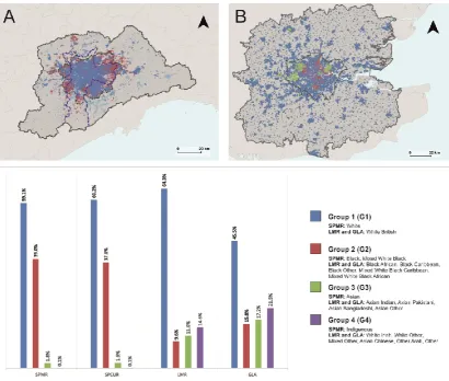
For comparability, the two areas would ideally be of similar size and population. While the two city authority extents - Greater London Authority (GLA) and São Paulo municipality (SPM) - are similar in area, SPM is more populous (11.2m in 2010, compared to 8.2m in 2011 in GLA) and is notable for the degree to which the continuous urban agglomeration extends beyond the municipal boundary. The SPMR has a population of 19.6m in 2010 (IBGE, 2010) in an area of 7,944km2. In comparison to LMR which presents mostly lower densities and is sprawled and sparse, in particular outside the GLA, the SPMR’s urban form is very dense and compact (see Figure 1). Given such different characteristics, LMR was defined based on a 10% commuting threshold to the GLA. The resulting area is shown in Figure1B (full line). The resulting area is shown in Figure 1(b) (full line), which has comparable population to the SPMR but a much larger area (15.95m people within 16,371km2 of area).
Although SPM has an area comparable to GLA, its boundaries divided the urban agglomeration as well as included non-urban areas which deemed it unsuitable for the analysis (see blue boundary in Figure1A). Thus, a newly defined area for SP was created based on the selection of continuous urban areas. This region, which has an area of 1,499 km2 and a population of 16.15m people, will be referred to here as the São Paulo Continuous Urban Region (SPCUR) and can be seen in Figure1A represented by the grey dashed line. It is interesting to note that SPCUR, in addition to be comparable in area to the GLA can also be considered as comparable in terms of population size with the LMR.
Definition of grouping systems
The definition of grouping systems for segregation measurement is usually done on an ad hoc basis depending on the objectives of a particular study as well as characteristics and regional traditions of a particular world region. By and large, there is great variation on the number and classes chosen for segregation studies, in particular for ethno-racial analysis. With few exceptions (for an example see Catney, 2017), a reduced number of classes is usually used in order to facilitate the analysis and interpretation. The criteria for such choices range greatly, with studies only analysing the most representative groups to clustering all available groups according to a set of criteria – which also varies. This often causes difficulties in the comparison between results across segregation studies for the same area.
a more detailed and ethnic-based classification system with 18 categories, which subdivides racial categories into ethnic origins and includes a number of mixed-groups classes (Office For National Statistics et al., 2016). Although both censuses present some common broader classes (Black, White, Mixed, Asian), differences in the ethno-racial composition between the study areas impose difficulties for the selection of compatible categories.
As the number of groups impacts directly on the results of the segregation indices adopted here, it is paramount to use the same number of groups for both São Paulo and London. While for Brazil it is standard practice to group mixed (Black and White) classes together with Black (Telles, 2006) grouping the large number of ethnic classes for London was more challenging as there are no standardised strategies used across existing studies. Although the broader classes from the UK Census seemed to offer a ready to use solution for the grouping problem, they were not equivalent to the Brazilian one. In particular, grouping different mixed classes of the UK Census together was not relevant for a spatial segregation study.
The solution adopted was to group ethno-racial classes based on their spatial location. With this objective, Pearson correlation and spatial autocorrelation (Moran’s Index) analyses were conducted in order to identify groups that present similar spatial patterns of residential location. The results obtained confirmed the choice for grouping mixed white and black groups together with Blacks for São Paulo, but classifying those sub-groups in a different way for London. For London, the White British class was kept as a separate category, all Black and Mixed Black classes were grouped together, South Asian classes (Indian, Bangladeshi and Pakistani) composed a third category, and a forth category was created with the remaining groups, with the exception of White Gypsy class which was removed from the analysis. Based on those results, categories of both censuses were grouped into four major groups: White (G1), Black (G2), Asian (G3) and Others (G4)1, as detailed in Figure 1. Since the under representation of G3 and G4 in the SPRM can have an effect on the segregation metrics results, additional analyses were conducted using two groups: G1 (‘White’ for SPMR and ‘British White’ for LMR) and G5 (composed by all other groups, that is, ‘Non-White’ or ‘Non-British White’).
As illustrated in the maps A and B in Figure 1, in all study areas, the predominant group is G1 (White or British Whites), with a majority of around 60% in SPMR and SPCUR, 64.3% in LMR, and 45.5% in the GLA. Both study areas of São Paulo have a second major predominant group in G2 (Black and Mixed) which, together with G1, make up over 98% of the population. In the case of London, both LMR and GLA are characterized by a greater presence of other ethno-racial groups, which in the case of the GLA make up to the majority of the population (see histogram in Figure 1).
Figure 1: Group preponderance maps for SPMR (A) and LMR (B) and histograms of population composition for the four geographical areas under study (SPMR, SPCUR, LMR and GLA).
4. Segregation in the Metropolitan Regions of São Paulo and
London: A Sensitivity Analysis
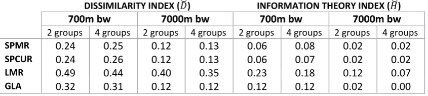
Global and local spatial indices of segregation depicting the spatial dimension evenness/clustering were calculated for London and São Paulo. The sensitivity of the indices D and H are tested in this section for three distinct aspects: grouping system (four and two ethno-racial groups), definition of geographical areas (SPMR, SPCUR, LMR and GLA), and scale (700m and 7000m bandwidths - bw). Table 2 presents the global spatial indices of generalized dissimilarity (𝐷̆) and information theory (𝐻̆) computed for these different research design options.
Table 2 – Global spatial indices of generalized dissimilarity (𝐷̆) and information theory (𝐻̆) computed for different areas (SPMR, SPCUR, LMR and GLA), grouping systems (two and four ethno-racial groups), and scales (700m and 7000m bw).
DISSIMILARITY INDEX (𝐷̆) INFORMATION THEORY INDEX (𝐻̆)
700m bw 7000m bw 700m bw 7000m bw
2 groups 4 groups 2 groups 4 groups 2 groups 4 groups 2 groups 4 groups
SPMR 0.24 0.25 0.12 0.13 0.06 0.08 0.02 0.02
SPCUR 0.24 0.26 0.12 0.13 0.06 0.07 0.02 0.02
LMR 0.49 0.44 0.40 0.35 0.23 0.18 0.12 0.07
GLA 0.32 0.31 0.12 0.12 0.12 0.12 0.02 0.00
Comparing the four geographic areas, it is worth noting the difference in results obtained for the different geographical areas definitions for London – LMR and GLA. The segregation levels of GLA are much lower than the ones obtained for LMR, especially at the 7000m scale. In contrast, the indices computed for São Paulo (SPMR and SPCUR) presented no clear difference between them.
When comparing all four areas, LMR stands out as the area with the highest levels of segregation, regardless of grouping or scale settings. The other three areas do not maintain a clear ranking order, as their results vary with the change of settings. For example, on a local scale (700m bw), GLA is more segregated than SPMR and SPCUR, regardless of the index or grouping system considered. Yet, the segregation levels of these three areas are very similar when calculated on a broader scale (7000m bw).
Comparing the results obtained for different grouping systems, LMR’s indices presented higher magnitude when computed for two groups, indicating the greatest imbalance in the spatial distribution of the LMR’s population occurs between G1 and G5. For the other areas (GLA, SPMR, SPCUR), the impact of the grouping systems on the results was much less expressive.
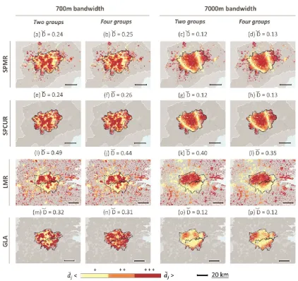
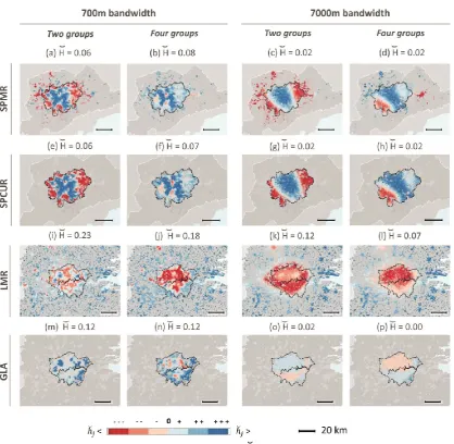
The results obtained with the global indices 𝐷̆ and 𝐻̆ are best understood through maps of local indices 𝑑̆𝑗 and ℎ̆𝑗, which show how each locality contributes to the overall composition of the global index. The maps shown in Figures 2 and 3 present the local indices 𝑑̆𝑗 and ℎ̆𝑗 of SPMR, SPCUR, LMR and GLA computed for
two scales (700 and 7000m) and two different grouping systems (two and four ethno-racial groups).
In the 𝑑̆𝑗 maps presented in Figure 2, darker areas represent localities with higher dissimilarity or, in other words, localities where the population composition differs from the overall population composition in the study area. While the index 𝑑̆𝑗
is always positive, the index ℎ̆𝑗 may assume positive or negative values. In the ℎ̆𝑗
[image:11.595.91.514.123.218.2]Figure 2: Local indices of generalized dissimilarity 𝑑̆𝑗 of SPMR, SPCUR, LMR and GLA (Gaussian function, 700m and 7000m bandwidth), computed for two and four ethno-racial groups.
It is noteworthy that the spatial pattern of dissimilarity seems almost insensitive to the definition of different grouping systems as the maps obtained for two and four ethno-racial groups present very similar spatial patterns. In both SPMR and LMR, it is possible to observe areas of high dissimilarity in both central and peripheral regions with an area of low dissimilarity in between, which act as a transition zone where the population composition tends to be closer to the metropolitan region as a whole. This configuration is particularly evident in the 7000m maps, which reveal broader patterns of segregation.
The most remarkable differences are noted between the different geographic definitions for London - LMR and GLA. While the 𝑑̆𝑗 indices computed for LMR
show the northern portion of GLA concentrating the most dissimilar areas, the
variations, the choice for one geographic definition or another may actually lead the analyst to very different conclusions.
Figure 3: Local indices of information theory ℎ̆𝑗 of SPMR, SPCUR, LMR and GLA (Gaussian function, 700m and 7000m bandwidth), computed for two and four ethno-racial groups.
Thus, the indices computed for the two-grouping system (G1 and G5) better depict SPMR’s and SPCUR’s reality and reveal patterns that match and complement those observed with the dissimilarity index (see, as example, Figures 2c and 3c). The
ℎ̆𝑗 indices provide new insights by revealing very different levels of diversity for areas
of high dissimilarity in SPMR’s central and peripheral regions. While the central areas are less diverse than the whole metropolis, due to the small presence of Non-Whites (in this case mainly Blacks), the outskirts of SPMR present a much more balanced composition of Whites and Non-Whites. The “transition zone” observed in the 𝑑̆𝑗 maps can also be identified in the ℎ̆𝑗 maps with light blue and red colours, which represent the localities where ℎ̆𝑗 is close to zero. Within the transition zone, 𝑑̆𝑗
and ℎ̆𝑗present low values because the locality’s population composition and entropy are closer to the ones observed for SPMR as a whole.
Despite the clear influence of the grouping system on the ℎ̆𝑗 indices of São Paulo, its sensitivity is more evident for London. In a comparison between the indices computed for LMR for two and four groups (Figures 3k and 3l, for example), the analysis for two groups shows the northern GLA as the least diverse region while the analysis for four groups reveals an inverse pattern. In the two-group classification, the low diversity of this region can be explained by the preponderance of Non-British White population. Yet, the four-group classification indicates the same region is highly diverse due to the balanced presence of British White, Black, Asian and Other (each group representing approximately 25%).
The four-group classification presents a more balanced distribution for London than São Paulo and, as such, provides a better representation of the ethno-racial diversity of the metropolis. Therefore, unlike São Paulo, the four-group ℎ̆𝑗 maps
reveal segregation patterns that are a closer match to those obtained with 𝑑̆𝑗 indices (see, for instance, Figures 2l e 3l).
In terms of the impact of geographical boundaries, looking at the maps presented in Figures 2 and 3, spatial patterns for SPMR and SPCUR for both 𝑑̆𝑗 and
ℎ̆𝑗 are visually very similar, while differences between spatial patterns for LMR and GLA are much more striking. The 𝑑̆𝑗 patterns for LMR and GLA are very distinct, while their ℎ̆𝑗 patterns resemble one another.
In addition to the visual analysis of maps, a set of correlation analyses using Spearman’s rank coefficient was carried out to quantitatively assess the impact of using different geographical areas as well as grouping systems and scales in the local measurements 𝑑̆𝑗 and ℎ̆𝑗. Spearman’s rank correlation, applied to the spatial units
which are common between the datasets for each pair of geographical areas (SPCUR and SPMR / LMR and GLA), allowed for the degree of the impact to be quantified as well as its nature to be further explored.
Table 3 shows Spearman’s coefficients for results of 𝑑̆𝑗 and ℎ̆𝑗 obtained using
obtained for São Paulo, with little evidence of impact due to change of geographical delimitation. For London, however, correlations range between weak and very strong. Also in agreement with the maps, London’s correlations for 𝑑̆𝑗 are much lower than for ℎ̆𝑗 suggesting 𝑑̆𝑗 has a higher sensitivity to changes in geographical areas than ℎ̆𝑗.
Table 3 Comparing local measurements for different geographical regions using Spearman correlation coefficient.
COMPARING GEOGRAPHIC REGIONS – SPEARMAN CORRELATION (SPCUR vs SPMR / GLA vs LMR)
Dissimilarity (𝑑̆𝑗) Information Theory (ℎ̆𝑗) São Paulo
SPCUR vs SPMR
London
GLA vs LMR
São Paulo
SPCUR vs SPMR
London
GLA vs LMR
bw=700m – 4 Groups 0.989 0.454 0.999 0.918
bw=7000m – 4 Groups 0.974 0.394 0.995 0.831
bw=700m – 2 Groups 0.988 0.263 0.997 0.972
bw=7000m – 2 Groups 0.972 0.313 0.998 0.549
All correlations are significant at the 0.01 level (2-tailed)
Spearman’s correlation was also carried out for the results obtained with different grouping systems (see Table 4), resulting in positive and very strong correlation coefficients for 𝑑̆𝑗 across all experiments. In comparison, results for ℎ̆𝑗
revealed a much greater variation and a high sensitivity of the local theory of information index to the grouping system employed, which is particularly evident for London. In the case of GLA, ℎ̆𝑗 indices calculated for the 7000m scale revealed a strong negative Spearman’s correlation (rs = -0.812). This can be observed in Figures
3o and 3q, which present inverted patterns. The two-groups map depicts a diverse south and a non-diverse north, while the four-groups map shows the opposite. Although less evident, the other grouping comparisons for London also reveal different ℎ̆𝑗 patterns, which were quantitatively captured by the weak correlations (rs
ranging from 0.045 to 0.104).
Table 4 Comparing local measurements for different grouping systems using Spearman correlation coefficient.
COMPARING GROUPING SYSTEMS – SPEARMAN CORRELATION (4 Groups vs. 2 Groups)
Dissimilarity (𝑑̆𝑗) Information Theory (ℎ̆𝑗) São Paulo
4 vs 2 groups
London 4 vs 2 groups
São Paulo 4 vs 2 groups
London 4 vs 2 groups
SPCUR/GLA – bw = 700m 0.986 0.869 0.523 0.093
SPCUR/GLA – bw = 7000m 0.996 0.827 0.679 -0.812
SPMR/LMR – bw = 700m 0.986 0.979 0.537 0.104
SPMR/LMR – bw = 7000m 0.996 0.999 0.700 0.045
Spearman’s correlation analysis was also carried out for the comparison of local measurements obtained using different bandwidths (700m vs. 7000m), as shown in Table . It is interesting to note the correlation levels between results obtained with two different bandwidths tend to be lower than in the previous two tables, demonstrating the impact of using different bandwidths on local measurements. This highlights the importance of conducting multiscale analysis of segregation, and confirms a spatial unit can be considered highly segregated in one scale and not in another (Catney, 2017; Fowler, 2016).
The comparison between scales does not allow the identification of which index is more sensitive to changes in scale. Nevertheless, the weak correlations of ℎ̆𝑗
for GLA and LMR when only two groups were considered (rs=0.223 and 0.205, respectively) reinforce previous findings concerning the sensitivity of ℎ̆𝑗 to grouping systems.
Table 5 Comparing local measurements for different bandwidths using Spearman correlation coefficient.
COMPARING SCALES – SPEARMAN CORRELATION (Bandwidths 700m vs. 7000m)
Dissimilarity (𝑑̆𝑗) Information Theory (ℎ̆𝑗) São Paulo
700 vs. 7000m
London 700 vs. 7000m
São Paulo 700 vs. 7000m
London 700 vs. 7000m
SPCUR/GLA – 4 Groups 0.641 0.624 0.508 0.582
SPMR/LMR – 4 Groups 0.634 0.684 0.515 0.704
SPCUR/GLA – 2 Groups 0.600 0.522 0.701 0.223
SPMR/LMR – 2 Groups 0.594 0.642 0.694 0.205
All correlations are significant at the 0.01 level (2-tailed)
When comparing results of D and H, it is clear the first is more sensitive to different geographical areas while the second is more sensitive to the grouping system. In order to make sense of the results, it is important to note, although both indices compare differences between global and local population characteristics, they do it in distinct ways. While D considers a global empirical population composition (the one observed for the whole study area) as reference for analysing the localities; H considers an ideal population composition, which represents the maximum diversity (equal proportion for all population groups), for analysing global and local population compositions and then compares the level of diversity between the localities and the whole. As such, the reference population composition used by H will not be affected by changes in the geographical boundaries unless the number of groups is altered as a consequence of changes in the boundaries.
very different population compositions, with the GLA concentrating much of the non-White British population of the LMR.
On the overall, the Spearman’s correlation analyses have quantified the impact caused by research design choices and revealed changes in global results are not uniformly distributed on local areas. In other words, the analysis showed the impact of those changes may not be on the order of magnitude of segregation across the whole geographical region (global indices) but rather on the segregation levels relative rank order of spatial units (local indices).
Thus, the conducted experiments reinforce the relevance of measuring segregation using both global and local indices. Only local indices are able to reveal certain variations relative not only to spatial patterns of segregation, but also to the different aspects of segregation that each index is capable of representing.
5. Conclusions
Since the publication of the first studies measuring segregation, continuous progress has been made in this field. Recent developments include the propositions of spatial global and local versions of traditionally used segregation indices, which have allowed an increasing number of studies to analyse segregation as a multiscale and spatially-varying phenomenon. Such studies tend to focus on urban areas (Catney, 2017) within specific geographical boundaries. Yet, the influence of research design choices, such as the extent of geographical boundaries, grouping systems and scales of analysis, on the measurement of segregation has been little explored to date. The present paper contributes in this direction by investigating the impact of such decisions in the outcomes of the indices of generalized dissimilarity (D) and information theory (H) and highlighting issues that should be taken into consideration when making those decisions as well as interpreting the results.
Experiments with spatial global and local versions of D and H have shown that although both indices depict the same spatial dimension of segregation (evenness/clustering), they have different levels of sensitivity to geographical extent and grouping systems. While D is more sensitive to differences in geographical extents, H is more sensitive to grouping systems. The latter had been previously highlighted by Peach (2009, p. 7) who argued that different grouping systems could be used to manipulate results “to increase or decrease the degree of diversity”. As the popularity of H increases, in particular due to its ability to depict segregation (evenness/clustering dimension) in relation to diversity, it becomes important to raise awareness to its sensitivity to the grouping system.
where White-British is majority makes the definition of London’s metropolitan boundaries much more problematic than for São Paulo.
The present study also demonstrated the importance of combining the use of global and local measures. H’s sensitivity to grouping systems, while masked by global indexes, was clearly revealed when mapping results of local indices and confirmed by Spearman’s correlation analyses. Mapping local indices also contributed to highlight the distinctions between D and H. While 𝑑̆𝑗 is only capable of
discriminating the localities whose population composition is more/less similar to the population composition of the whole, ℎ̆𝑗 provides a more informative representation of segregation. Its range from negative to positive values, which is hidden in the overall global index, allows the differentiation of areas with higher or lower diversity than the study area.
While the existent literature on the evaluation of different segregation indices focuses on theoretical rather than empirical approaches, this study contributes to a better understanding of the impact of research design choices such as grouping systems and geographical boundaries in applied studies. Applying the same methodology for different areas in a comparative fashion allowed for nuances of D and H, two widely-used evenness/clustering measures, to be revealed. It became clear each index requires specific attention to research design choices and to the meaning of their outputs. Despite representing the same spatial dimension, their results are far from being interchangeable.
Acknowledgements
The authors would like to thank the editors and anonymous reviewers from this journal for their insightful and useful feedback on earlier versions of this article. They would also like to thank all partners in the RESOLUTION Project for their contributions to this research.
All datasets used in this article are open and available for download from the UK (table ‘KS201EW’) and Brazil (table ‘Pessoa03UF’) censuses websites. All segregation indices were calculated in QGIS using the SEGREG Plugin (https://plugins.qgis.org/plugins/Segreg/) developed as part of the RESOLUTION Project.
Funding
References
Catney, G., 2017. The complex geographies of ethnic residential segregation: using spatial and local measures to explore scale-dependency and spatial relationships. Transactions of the Institute of British Geographers. https://doi.org/10.1111/tran.12209
Clark, W.A.V., Anderson, E., Östh, J., Malmberg, B., 2015. A Multiscalar Analysis of Neighborhood Composition in Los Angeles, 2000–2010: A Location-Based Approach to Segregation and Diversity. Annals of the Association of
American Geographers 105, 1260–1284.
https://doi.org/10.1080/00045608.2015.1072790
Duncan, O.D., Duncan, B., 1955. A Methodological Analysis of Segregation Indexes. American Sociological Review 20, 210. https://doi.org/10.2307/2088328 Feitosa, F.F., Câmara, G., Monteiro, A.M.V., Koschitzki, T., Silva, M.P.S., 2007.
Global and local spatial indices of urban segregation. International Journal of
Geographical Information Science 21, 299–323.
https://doi.org/10.1080/13658810600911903
Fowler, C.S., 2016. Segregation as a multiscalar phenomenon and its implications for neighborhood-scale research: the case of South Seattle 1990?2010. Urban Geography 37, 1–25. https://doi.org/10.1080/02723638.2015.1043775
IBGE, 2010. 2010 Census. Brazil.
Johnston, R., Poulsen, M., Forrest, J., 2007. The Geography of Ethnic Residential Segregation: A Comparative Study of Five Countries. Annals of the Association of American Geographers 97, 713–738. https://doi.org/10.1111/j.1467-8306.2007.00579.x
Lloyd, C.D., Shuttleworth, I., 2012. Residential Segregation in Northern Ireland in 2001: Assessing the Value of Exploring Spatial Variations. Environment and Planning A 44, 52–67. https://doi.org/10.1068/a44167
Massey, D.S., Denton, N.A., 1988. Suburbanization and segregation in US metropolitan areas. American Journal of Sociology 94, 592–626.
Mateos, P., 2015. The international comparability of ethnicity classifications and its consequences for segregation Studies, in: Lloyd, C.D., Shuttleworth, I., Wong, D.W.S. (Eds.), Social-Spatial Segregation: Concepts, Processes and Outcomes. Policy Press, Bristol.
Office For National Statistics, National Records Of Scotland, Northern Ireland Statistics And Research Agency, 2016. 2011 Census aggegate data (Data downloaded: 1 June 2016). https://doi.org/10.5257/census/aggregate-2011-1 Östh, J., Clark, W.A.V., Malmberg, B., 2015. Measuring the Scale of Segregation
Using k -Nearest Neighbor Aggregates: Measuring the Scale of Segregation. Geographical Analysis 47, 34–49. https://doi.org/10.1111/gean.12053
O’Sullivan, D., Wong, D.W., 2007. A Surface-Based Approach to Measuring Spatial Segregation. Geographical Analysis 39, 147–168.
Peach, C., 2009. Slippery segregation: discovering or manufacturing ghettos? Journal of Ethnic and Migration Studies 35, 1381–1395.
Poulsen, M., Johnson, R., Forrest, J., 2002. Plural Cities and Ethnic Enclaves: Introducing a Measurement Procedure for Comparative Study. International Journal of Urban and Regional Research 26, 229–243. https://doi.org/10.1111/1468-2427.00377
Methods in Social Epidemiology. Jossey-Bass, San Francisco, CA, pp. 169– 192.
Reardon, S.F., Firebaugh, G., 2002. Measures of multigroup segregation. Sociological methodology 32, 33–67.
Reardon, S.F., Matthews, S.A., O’Sullivan, D., Lee, B.A., Firebaugh, G., Farrell, C.R., Bischoff, K., 2008. The geographic scale of metropolitan racial segregation. Demography 45, 489–514.
Reardon, S.F., O’Sullivan, D., 2004. Measures of spatial segregation. Sociological methodology 34, 121–162.
Sakoda, J.M., 1981. A Generalized Index of Dissimilarity. Demography 18, 245. https://doi.org/10.2307/2061096
Theil, H., Finizza, A.J., 1971. A note on the measurement of racial integration of schools by means of informational concepts. The Journal of Mathematical Sociology 1, 187–193. https://doi.org/10.1080/0022250X.1971.9989795 Voas, D., Williamson, P., 2000. The Scale of Dissimilarity: Concepts, Measurement
and an Application to Socio-Economic Variation across England and Wales. Transactions of the Institute of British Geographers 25, 465–481.
White, M.J., 1983. The measurement of spatial segregation. American journal of sociology 88, 1008–1018.