The Self Calibration Method for Multiple Systems at the CHARA Array

(1)

ScholarWorks @ Georgia State University

Mathematics Theses Department of Mathematics and Statistics

Spring 4-18-2011

Stability Selection of the Number of Clusters

Gabriella v. Reizer

Follow this and additional works at: https://scholarworks.gsu.edu/math_theses Part of the Mathematics Commons

Recommended Citation Recommended Citation

Reizer, Gabriella v., "Stability Selection of the Number of Clusters." Thesis, Georgia State University, 2011. https://scholarworks.gsu.edu/math_theses/98

This Thesis is brought to you for free and open access by the Department of Mathematics and Statistics at ScholarWorks @ Georgia State University. It has been accepted for inclusion in Mathematics Theses by an authorized administrator of ScholarWorks @ Georgia State University. For more information, please contact

(2)

STABILITY SELECTION OF THE NUMBER OF CLUSTERS

by

GABRIELLA VALERIA REIZER

Under the Direction of Yixin Fang

ABSTRACT

Selecting the number of clusters is one of the greatest challenges in clustering analysis. In this

thesis, we propose a variety of stability selection criteria based on cross validation for determining the

number of clusters. Clustering stability measures the agreement of clusterings obtained by applying the

same clustering algorithm on multiple independent and identically distributed samples. We propose to

measure the clustering stability by the correlation between two clustering functions. These criteria are

motivated by the concept of clustering instability proposed by Wang (2010), which is based on a form of

clustering distance. In addition, the effectiveness and robustness of the proposed methods are

numeri-cally demonstrated on a variety of simulated and real world samples.

(3)

by

A Thesis Submitted in Partial Fulfillment of the Requirements for the Degree of

Master of Science

in the College of Arts and Sciences

Georgia State University

(4)

Copyright by Gabriella Valeria Reizer

(5)

by

Committee Chair: Dr. Yixin Fang

Committee: Dr. Gengsheng Qin

Dr. Ruiyan Luo

Electronic Version Approved:

Office of Graduate Studies

College of Arts and Sciences

Georgia State University

(6)

DEDICATION

To my husband, Catalin.

“Love is patient, love is kind. It does not envy, it does not boast, it is not proud. It is not rude, it is not

self-seeking, it is not easily angered; it keeps no record of wrongs. Love does not delight in evil but

re-joices with the truth. It always protects, always trusts, always hopes, always perseveres. Love never

fails.”

(7)

ACKNOWLEDGEMENTS

First and foremost I would like to offer my sincerest gratitude to my advisor, Dr. Yixin Fang, who

has supported me throughout my thesis with his patience and knowledge. This thesis would not have

been possible without his guidance.

I would like to thank Dr. Junhui Wang at University of Illinois at Chicago for the thoughtful

dis-cussion and for his generosity for sharing the R-codes.

I would like to thank my committee members Dr. Jeff Qin and Dr. Ruiyan Luo for accepting my

invitation and taking their time to read my thesis. I appreciate all their insightful comments and their

encouragements.

I would also like to acknowledge all my professors in the Mathematics and Statistics

Depart-ment at Georgia State University for sharing with me their precious statistical knowledge and skills and

for all their assistance along the years.

Last but not the least; I would like to express my deepest gratitude to my family for supporting

me through my studies. My greatest thanks go to my loving and encouraging husband. It has been a

(8)

TABLE OF CONTENTS

ACKNOWLEDGEMENTS ... v

LIST OF TABLES ... viii

LIST OF FIGURES ... ix

CHAPTER 1 INTRODUCTION ... 1

1.1 Clustering methods ... 1

1.1.1 K-means clustering ... 1

1.1.2 Hierarchical clustering ... 3

1.1.3 Spectral clustering ... 5

1.2 Determining the number of clusters in a dataset ... 6

1.3 Existing methods for selecting the number of clusters... 6

1.4 Literature on clustering stability ... 7

1.5 Instability selection of the number of clusters ... 8

1.6 Stability selection of the number of clusters ... 9

1.7 Summary ... 10

CHAPTER 2 CLUSTERING INSTABILITY ... 11

2.1 Introduction ... 11

2.2 Instability ... 12

2.3 Cross-validation for clustering ... 13

2.3.1 Cross-validation with voting ... 14

2.3.2 Cross-validation with averaging ... 15

(9)

CHAPTER 3 CLUSTERING STABILITY... 16

3.2 Stability ... 17

3.3 Cross-validation for clustering ... 17

3.3.1 Cross-validation with voting ... 18

3.3.2 Cross-validation with averaging ... 18

CHAPTER 4 SELECTION CONSISTENCY ... 20

CHAPTER 5 NUMERICAL EXPERIMETS ... 23

5.2 Simulated examples ... 23

5.2.1 Two-dimensional examples ... 23

5.2.2 Multi-dimensional examples ... 27

5.3 Real examples ... 29

CHAPTER 6 DISCUSSION ... 31

REFERENCES ... 32

(10)

LIST OF TABLES

Table 5.1. Two-dimensional examples: the estimated numbers of clusters using stability and

instability ……… 26

Table 5.2. Multi-dimensional examples: the estimated numbers of clusters using stability

(11)

LIST OF FIGURES

Figure 1.1 An illustrative example on clustering instability and stability ... 9

Figure 5.1 Two-dimensional examples ... 24

Figure 5.2 Estimated clustering stability and instability for Example 7 ... 28

Figure 5.3 Estimated clustering stability and instability for the wine data ... 29

(12)

Chapter 1

Introduction

1.1 Clustering Methods

Clustering analysis, also called data segmentation, is the process of assigning a set of

observa-tions to groups (clusters) so that the items in a cluster are similar in some sense (but not identical) to

one another and very different from the items in other clusters.

Usually, clustering analysis is based on measures of distances between objects being clustered.

We introduce here three of the most known clustering methods: k-means clustering, hierarchical

clus-tering and spectral clusclus-tering.

1.1.1 K-means clustering

The idea of k-means goes back to Hugo Steinhaus in 1956, but the actual term was first used by

James MacQueen in 1967.

In clustering analysis it is assumed that zn =( ,...,x₁ xn)are independently sampled from some

unknown distribution p x( ) withx∈ℝp. This non-hierarchical approach aims to partition the n

p-dimensional observations into k clusters (

k

≤

n

) by minimizing a measure of dispersion within the

clusters. The most common measure used is the sum of squared distances between all points and the

cluster centers.

The first step of the process is to choose the k initial cluster centers. It is really important to run

(13)

place the centroids as far away from each other as possible. The next step is to take each point and

as-sociate it with the closest center. At this point all k centroids are recalculated and the process stars

over. Note that the k centroids change their location each time until no more changes are made.

Therefore, the algorithm aims to minimize an objective function:

2 ( ) 1 1

,

= =

=

∑∑

k n j −

i j

j i

J x c

where

_i

is a distance between two data points.

The k-means algorithm

Step 1. The data set is divided randomly into k clusters that have roughly the same number of data

points.

Step 2. For each data point the distance to each cluster is calculated. If the data point is closest to its

own cluster, the data point is left where it was. If the data point is not closer to its own cluster, the data

point is associated to the closest cluster.

Step 3. Repeat the above step until a complete pass through all the data points results in no data point

moving from one cluster to another. At this point the clusters are stable and the clustering process ends.

The initial cluster selection can greatly affect the final clusters that result, in terms of

inter-cluster and intrainter-cluster distances and cohesion.

The advantages of the k-means algorithm are as follows: each cluster contains at least one data

point, there are exactly k clusters, the clusters are non-hierarchical, and it can be applied to large data

(14)

1.1.2. Hierarchical clustering

Hierarchical clustering focuses on forcing the data points into a strict hierarchy of nested

sub-sets. Lance and Williams in 1967 discuss a large variety of hierarchical clustering algorithms. The results

of a hierarchical method can be displayed in a tree diagram, known as dendrogram.

In comparison to k-means (a non-hierarchical clustering method), in hierarchical clustering the

data are not partitioned into k clusters in step one. This method does not require an initial value for k,

which can be considered an advantage. Despite this advantage the hierarchical clustering seems to be

less efficient compared to k-means.

There are two well known types of hierarchical clustering methods: agglomerative hierarchical

clustering or the “bottom up” approach, which proceeds by a series of fusions of the n data points into

groups, and divisive hierarchical clustering or the “top down” approach, which separates recursively as

one moves down the hierarchy the n data points into finer groupings

Agglomerative hierarchical clustering

This method starts with as many clusters as data points and in each successive iteration, it

ag-glomerates the closest two clusters that satisfy a predefined similarity criteria. Clusters are successively

merged until only one cluster remains.

The Agglomerative hierarchical clustering algorithm:

Step 1.n clusters are created; each data point is assigned to a separate cluster. Then, all the distances

between clusters are calculated and a symmetric matrix of distances (similarities) is constructed.

Step 2. The shortest distance within two clusters is obtained.

(15)

Step 4. Repeat Steps 2 and 3n-1 times (until the distance matrix is reduced to a single element).

The agglomerative hierarchical clustering produces an ordering of the objects (informative for

data display). Different distance metrics may generate different results. Performing multiple

experi-ments and comparing the results is recommended to support the veracity of the original results. Small

number of clusters is obtained, property that can be really helpful for discovery. No provision can be

made for a relocation of objects that may have been 'incorrectly' grouped at an early stage. The result

should be examined closely to ensure that it makes sense.

Divisive hierarchical clustering

This top-down clustering method is less commonly used. It works in a similar way to the

agglo-merative clustering but backwards. It starts with only one big cluster formed by all data points and in

each successive iteration groups are continually divided until there are as many clusters as objects.

The divisive hierarchical clustering algorithm:

Step 1. One big cluster containing all data points is initially considered. All the distances between points

are calculated and the symmetric matrix of distances (dissimilarities) constructed.

Step 2.The longest distance within two data points/clusters is obtained.

Step 3. The data is divided into two clusters and the distance matrix updated.

Step 4. Repeat Steps 2 and 3n-1 times.

The top down hierarchical clustering is conceptually more complex that the bottom up

cluster-ing, since it needs a second clustering algorithm as a “subroutine”. It’s been proven that produces more

accurate hierarchies than the bottom up algorithms in some circumstances. Divisive hierarchical

(16)

decisions, while agglomerative hierarchical clustering methods make clustering decisions based on local

patterns without initially taking into account the global distribution.

1.1.3. Spectral clustering

Spectral clustering techniques rely on the eigenstructure of the matrices derived from the data. It

parti-tions points into disjoint clusters with points in the same clusters having high similarity and points in

dif-ferent clusters having low similarity.

The Normalized Cuts algorithm by Shi and Malik (1997) is frequently used for image

segmenta-tion.

Spectral clustering it is simple to implement, and can be solved efficiently by any standard linear

algebra software. Ng, Jordan and Weiss (2001) proposed a simple spectral clustering algorithm that can

be implemented using a few lines of Matlab. They show surprising results on a number of challenging

clustering situations, proving that spectral clustering can outperform traditional clustering algorithms

(such as k-means).

The spectral clustering algorithm

Step 1. The affinity matrix and the diagonal matrix are created.

Step 2. The largest eigenvector is created (chosen to be orthogonal to each other in the case of repeated

eigen values) and a new matrix in created by stacking the eigenvectors in columns.

Step 3. Each row of the matrix is renormalized to have unit length.

Step 4. Treating each row of the new matrix as a point, k clusters are created via any clustering

(17)

Step 5. Finally, each original point is assigned to a cluster if and only if the corresponding row of the

ma-trix was assigned to a cluster.

1.2 Determining the number of clusters in a data set

The concept of the number of clusters is very different between hierarchical and partitional

clus-tering algorithms. In the case of hierarchical clusclus-tering, the number of clusters does not necessarily need

to be specified beforehand. This number can vary depending on the level the tree is cut. On the other

hand, partitional clustering requires that the number of clusters be specified before the algorithm is

per-formed.

The selection of an appropriate number of clusters, quality often labeled as k(as in the k-means

algorithm), is one of the most difficult problem in clustering analysis. Traditionally the value of k is

ob-tained by performing a clustering algorithm with several different values of k and selecting the one that

leads to the optimal clusterings. It is clear that this is a trial and error process. For small datasets this is

not a significant problem. However, for large datasets this can be very time consuming.

If an appropriate value of k cannot be determined from prior knowledge of the dataset, some

other method has to be chosen. The absence of an objective measure that examines the quality of the

clusterings of a particular dataset makes the process of selecting a correct k an even harder task. Several

decision making methods are available to us.

1.3. Existing methods for selecting the number of clusters.

There are many methods available to estimate the number of clusters these days. Several of

these approaches were analyzed by Milligan and Cooper (1985) and by Dubes (1987). Rissanen (2000)

(18)

pa-nelized that the less complex ones. Other methods, such as Akaike Information Criterion (AIC) proposed

by Akaike (1974) and Schwartz Information Criterion (SIC) derived by Schwarz (1978) are considered

op-timum for selecting the number of clusters for high-model complexity.

MDL (Rissanen 1996), AIC (Akaike, 1974), BIC and SIC (Schwarz, 1978) are some examples of

pe-nalized likelihood estimation methods. Resampling attempts to find the appropriate number of clusters

by clustering many data samples, and determining where clusterings are “most stable”.

Cross-validation is another approach for estimating the number of clusters proposed by Smyth

(1996). This method splits the data in two or more parts. One part is used for clustering and the other

part(s) is used for validation. Monte Carlo cross-validation attempts to fit the data quite accurately but

in the same time minimizes the complexity of the model.

1.4. Literature on clustering stability

Another widely used method for selecting the number of clusters is based on stability

argu-ments: the number of clusters is chosen so that the corresponding clustering results are “most stable”.

In recent year, several papers have been written on this method from the theoretical point of view.

The idea behind clustering stability is that a “good” algorithm tends to repeatedly produce

simi-lar clusterings on data originating from the same source. In other words, the algorithm is stable with

respect to input randomization.

A major issue, as pointed out by Krieger and Green (1999) is that a clustering model is stable

on-ly if the objective function has a unique global minimize. It is demonstrated that the approaches

men-tioned in the article, fail to determine the appropriate number of clusters, especially if the sample size

gets larger and the variable exhibit higher correlation. The clustering stability might not be that desirable

(19)

Ben-Hur, Elisseeff and Guyon (2002) propose to use distribution of pairwise similarity between

clusterings of sub-samples of a dataset as a measure of the stability of a partition. In this paper several

experiments are run, and all the results coincide with the intuitive selection.

Lange, Roth, Braun and Buhmann (2004) proposed a new measure of clustering stability to

as-sess the validity of a cluster model. Good performances have been achieved on both, simulated data

and gene expression data sets.

Another great paper on this idea is presented by Ben-David, von Luxburg and Pal (2006). In this

work, the authors propose some new definitions of stability and some related clustering notions. The

results suggest that the existence of a unique minimize indicates stability, and the existence of a

symme-try permuting such minimize indicates instability. The results indicate that stability does not reflect the

validity or meaningfulness of the selection of the number of clusters. Instead, the parameters it

meas-ures are independent of clustering parameters.

1.5. Instability selection of the number of clusters

Wang (2010) focuses in his paper on introducing some novel criteria for determining the

num-ber of clusters. This new selection criterion measures the quality of clusterings through their instability

from sample to sample. Here the clustering instability is estimated through cross validation, and the goal

of the method is to minimize the instability. The data is divided into two training sets and one validation

set to imitate the definition of stability. Then, a distance based clustering algorithm is applied on the

independent and identically distributed training sets and the inconsistencies evaluated on the validation

set. This method has been proven to be effective and robust on a variety of simulated and real life

(20)

[image:20.612.94.499.95.500.2]

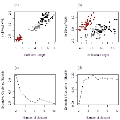
Selection of the number of clusters for the iris data.

Figure 1.1 An illustrative example on clustering instability and stability: (a) the iris data – Petal; (b) the iris data – Sepal; (c) clustering stability curve; (d) clustering instability curve

1.6. Stability selection of the number of clusters

In this thesis, we propose a novel definition of stability. To measure the clustering stability we

(21)

found in Fowlkes and Mallows (1983), where similarly the closeness between two hierarchical clustering

functions is used.

The stability measure is assumption free and applicable to the distance based clustering

algo-rithm described by Wang, and also applicable to the non-distance based clustering algoalgo-rithms.

By definition, the clustering stability serves as a quality measure of the clustering algorithm, so it

can be used to compare clusterings with different numbers of clusters. The well known iris data is used

to demonstrate how the number of clusters changes the stability measure; and the results are displayed

in Figure 1.1. Evidently, the maximum clustering stability and the minimum clustering instability are

achieved at k=2. The iris data is one of the examples in Chapter 5, while Chapter 3 in dedicated entirely

to our novel method of determining the number of clusters by maximizing the stability.

1.7. Summary

The rest of this thesis is organized as follows. Chapter 2 presents the definition of instability

based on the distance proposed by Wang (2010). Chapter 3 introduces the newly proposed definition of

stability based on correlation. Chapter 4 focuses on selection consistency. In Chapter 5 we compare the

two approaches on both simulated and real world examples. Finally, Chapter 6 contains some

(22)

Chapter 2

Clustering Instability

Most of the materials in this chapter are reproduced from Wang (2010).

2.1. Introduction

To introduce the definition of instability proposed by Wang (2010), we first define our variables.

We assume that

z

n

=

( ,

x x

₁ ₂

,...,

x

_n

)

is independently sampled from some known probability

distribu-tion p x( ) with p

x∈ℝ . In clustering analysis, a clustering is defined as a mapping

φ

( ; ,

⋅

k Z

n

)

:

{

1,...,

}

p

k

→

ℝ

, where φ and the number of clusters

k

≥

2

are predetermined.

The distance between two cluterings is defined by Wang (2010) as follows.

Definition 1 (Clustering Distance). For any two clusterings

φ

₁

( )

x

and

φ

₂

( )

x

of the same datazn, the

dis-tance between

φ

₁

( )

x

and

φ

₂

( )

x

is defined as

(

)

1 2 1 2

( ,

φ φ

)

=

+ =

1 ,

Dist

P I

I

where I( )⋅ is an indicator function,

I

₁

=

I

{

φ

₁

( )

X

=

φ

₁

( )

Y

}

and

I

₂

=

I

{

φ

₂

( )

X

=

φ

₂

( )

Y

}

and X and Y are

i.i.d. fromp x( ).

The distance function is required to satisfy the following conditions: non-negativity, identity of

indiscernibles, symmetry and subadditivity/triangle inequality. Ben-David, von Luxburg and Pal (2006)

have been established that the clustering distance has to be symmetrical and has to satisfy the triangle

(23)

1 2

( ,

)

0 Dist

φ φ

=

then

φ φ

₁

=

₂. As a prototypic example they considered the Hamming distance (or

pair-counting distance).

In a similar way, Wang proves that the distance proposed d( , )⋅ ⋅ is a legitimate distance

meas-ure. Wang proves that the distance is nonnegative, symmetrical and satisfies the triangle inequality.

2.2. Instability

Wang’s definition of instability of a clustering algorithmφ as the expected distance of two

clus-terings obtained by applying φ to two i.i.d. samples from p x( ) with a given number of clusters is as

fol-lows.

Definition 2 (Clustering Instability). Given the number of clusters k, the instability of φ is defined as

*

( , )

(

( ( ; ,

n

), ( ; ,

n

)))

Instab

φ

k

=

E Dist

φ

⋅

k Z

φ

⋅

k Z

,

where

φ

( ; ,

⋅

k Z

n

)

and

φ

( ; ,

⋅

k Z

*n

)

are clusterings obtained by applying φ onZnand Z*nrespectively; and

n

Z and Z*nare two independent samples from p(x).

So, the clustering instability is actually a quality measure of any clustering algorithm. Wang

sug-gested the use of clustering instability to compare clusterings of a data set with different number of

clusters. If the number of clusters is greater than the true one, the clustering algorithm will split true

clusters into small one and this split changes from sample to sample; on the other hand if the number of

clusters is smaller than the true one, the algorithm will merge true clusters into bigger once and this

(24)

2.3. Cross validation for clustering

This technique is mainly used in settings where the goal is prediction, and the purpose of it is to

assess how the result of a statistical analysis will apply to a data set. So basically it can be considered as

a model selection criteria. Allen (1974), Stone (1974) and Geisser(1975) were the first once to dedicate

their time to cross validation.

Cross-validation is based on data splitting, part of the data being used to construct a model and

the rest of the data is used to measure the performance of the model. The first part of the data is called

the training set and the second part of the data is called the validation set.

The following cross validation techniques are worth to mention.

R-fold cross-validation (Breiman, 1984) partitions the data into r equally (or nearly equally) sized

segments or folds. One fold is used as a validation set and the rest as a training set. The process is

re-peated r times (until each fold is selected as validation set one time)

Multifold cross-validation (Zhang, 1993) considers all possible partitioning with the same ratio

and repeated learning-testing (Burman, 1989) considers only one subset of splittings with the same

ra-tio.

Wang focused his attention on the repeated learning-testing scheme in implementation

subse-quently. We are going to follow his lead and use the repeated learning-testing scheme as well. Because

of the multiple data splittings used in model selection, two different ways to help summarize the results

(25)

2.3.1. Cross-validation with voting

Let

{ ( ; ,

φ

⋅

k z

n

)}

be a set o clusters and k=2,…,K, where K is predetermined as the largest possible

num-ber of clusters in comparison. zn is split into two training sets and one validation set. Two clusterings

are created by applying the same algorithm φ on the two training sets, and the validation set is used to

measure the distance between the two clusterings. Then, the procedure that minimizes the instability in

each splitting is selected, and the procedure selected the most number of times is selected as the best

one. Note that this algorithm is applicable to any clustering method as long as the observations are

in-dependently and identically distributed.

Cross-validation with voting algorithm for clustering proposed by Wang:

Step1. Permute data

( ,...,

x

₁

x

_n

)

and obtain

(

x

₁*c

,...,

x

_n*c

)

.

Step2. Split the permuted data

(

x

₁*c

,...,

x

_n*c

)

into three parts with

m

,

m

and n−2mobservations

re-spectively:

z

₁*c

=

(

x

₁*c

,...,

x

_m*c

)

,

z

₂*c

=

(

x

_m₊₁*c

,...,

x

₂_m*c

)

and

z

₃*c

=

(

x

₂_m₊₁*c

,...,

x

_n*c

)

.

Step 3. For simplicity, let

(

* * * *

)

(

₍

(

* *

) (

* *

)

₎

₍

(

* *

) (

* *

)

₎

)

1 2 1 1 2 2

, ; , ,

φ

, =

φ

; , =

φ

; , +

φ

; , =

φ

; , =1 .

c c c c c c c c c c c c

i j i j i j

V x x k z z I I x k z x k z I x k z x k z

Then the estimated Instab( , )

φ

k is defined as

*

(

)

* * * *

1 2 2 1

( , )

φ

, ; , ,

φ

, .

+ ≤ < ≤

=

∑

c

c c c c

i j

m i j n

Instab k V x x k z z

Step 4. Compute kɵ*c =arg min₂_{≤ ≤}_{k K}

Instab

*c

( , )

φ

k

.

(26)

2.3.2. Cross-validation with averaging

This technique averages the instability measures over the different partitioning and selects the

procedure that yields the minimum averaged error.

Cross-validation with voting algorithm for clustering proposed by Wang:

Step1. Permute data

( ,...,

x

₁

x

_n

)

and obtain

(

x

₁*c

,...,

x

_n*c

)

.

(

x

₁*c

,...,

x

_n*c

)

m

,

m

re-spectively:

z

₁*c

=

(

x

₁*c

,...,

x

_m*c

)

,

z

₂*c

=

(

x

_m₊₁*c

,...,

x

₂_m*c

)

and

z

₃*c

=

(

x

₂_m₊₁*c

,...,

x

_n*c

)

.

(

* * * *

)

(

₍

(

* *

) (

* *

)

₎

₍

(

* *

) (

* *

)

₎

)

1 2 1 1 2 2

, ; , ,

φ

, =

φ

; , =

φ

; , +

φ

; , =

φ

; , =1 .

i j i j i j

Then the estimated Instab( , )

φ

k is defined as

*

(

)

* * * *

1 2 2 1

( , )

φ

, ; , ,

φ

, .

+ ≤ < ≤

=

∑

c

c c c c

i j

m i j n

Instab k V x x k z z

Step 4. Define

*

1

( , )

C _c

c

Instab

φ

k

C

−

Instab

φ

k

=

∑

, when c = 1, … C.

(27)

Chapter 3

Clustering Stability

3.1. Introduction

A clustering algorithm is considered a good algorithm if it produces clusterings that do not vary

much from one sample to another sample; if repeated samples are drawn.

In Chapter 2 we introduce Wang’s idea of instability based on a form of clustering distance. The

main idea of his method is to minimizing the instability.

In Chapter 3, we propose to measure the clustering stability by the correlation between two

clustering functions, similar to the one used to measure the closeness between two hierarchical

cluster-ing functions in Fowlkes and Mallows (1983).

Definition 3 (Clustering Correlation). For any two clusterings

φ

₁

( )

x

and

φ

₂

( )

x

of the same datazn, the

correlation between

φ

₁

( )

x

and

φ

₂

( )

x

is defined as

(

) (

)

(

)

(

)

(

)

(

)

1 2 1 2

1 2

1 1 2 2

1

1 ( ,

)

,

1 1

1 1 1

1 φ φ

=

= = −

=

−

=

−

=

P I

I

P I

Corr

P I

where

I

₁

=

I

{

φ

₁

( )

X

=

φ

₁

( )

Y

}

and

I

₂

=

I

{

φ

₂

( )

X

=

φ

₂

( )

Y

}

, and X and Y are i.i.d. fromp x( ).

(28)

Clearly, the clustering correlation defined above is closely related to Wang’s definition of the

clustering distance.

3.2. Stability

Our definition of stability of a clustering algorithm φ as the expected correlation between two

clustering functions obtained by applying φ to two i.i.d. samples from p x( ) with a given number of

clus-ters is as follows.

Definition 4 (Clustering Stability). Given the number of clusters k, the stability of any

φ

( ; ,

⋅

k Z

n

)

is

de-fined as

(

) (

)

(

)

{

*

}

( , )

; ,

n

,

; ,

n

Stab

φ

k

=

E Corr

φ

⋅

k Z

φ

⋅

k Z

,

where

φ

(

⋅; ,k Zn

)

and

φ

(

⋅; ,k Z*n

)

are clusterings obtained by applying φ onZnand Z*nrespectively;

and Znand Z*nare two independent samples from p(x).

3.3 Cross-validation for clustering

The key idea is the same as the one proposed by Wang. The data is divided into two training sets

and one validation set, where the two training sets are used to construct two clustering functions via the

same clustering algorithm, and the clustering stability is calculated as the correlation between the two

clustering measured on the validation set. Multiple data splittings are performed in order to reduce

(29)

As discussed in Chapter 2, there are two ways to perform multiple data splittings; one is called

cross validation with voting and the other is called cross-validation with averaging. We will describe both

in the following.

3.3.1. Cross-validation with voting

Cross validation with voting algorithm for clustering using the newly defined stability:

Step1. Permute data

( ,...,

x

₁

x

_n

)

and obtain

(

x

₁*c

,...,

x

_n*c

)

.

(

x

₁*c

,...,

x

_n*c

)

m

,

m

re-spectively:

z

₁*c

=

(

x

₁*c

,...,

x

_m*c

)

,

z

₂*c

=

(

x

_m₊₁*c

,...,

x

₂_m*c

)

and

z

₃*c

=

(

x

₂_m₊₁*c

,...,

x

_n*c

)

.

(

* * * *

)

(

* *

) (

* *

)

(

* *

) (

* *

)

1 2 1 1 2 2

, ; , ,

φ

, =

φ

; , =

φ

; , +

φ

; , =

φ

; , =1 .

i j i j i j

Then the estimated

Stab

( , )

φ

k

is defined as

*

(

* * * *

)

1 2 2 1

( , )

φ

, ; , ,

φ

, .

+ ≤ < ≤

=

∑

c

c c c c

i j

m i j n

Stab k V x x k z z

Step 4. Compute kɵ*c =arg max₂_{≤ ≤}_{k K}

Stab

*c

( , )

φ

k

.

Step 5. Repeat Steps 1-4 for c = 1, … C, and define

k

ɵ

as the mode of

{

kɵ*1,kɵ*2,...,kɵ*C

}

.

3.3.2. Cross validation with averaging

This technique averages the stability measure over the different partitioning and selects the

(30)

Cross validation with averaging algorithm for clustering using the newly defined stability:

Step1. Permute data

( ,...,

x

₁

x

_n

)

and obtain

(

x

₁*c

,...,

x

_n*c

)

.

(

x

₁*c

,...,

x

_n*c

)

m

,

m

re-spectively:

z

₁*c

=

(

x

₁*c

,...,

x

_m*c

)

,

z

₂*c

=

(

x

_m₊₁*c

,...,

x

₂_m*c

)

and

z

₃*c

=

(

x

₂_m₊₁*c

,...,

x

_n*c

)

.

(

* * * *

)

(

₍

(

* *

) (

* *

)

₎

₍

(

* *

) (

* *

)

₎

)

1 2 1 1 2 2

, ; , ,

φ

, =

φ

; , =

φ

; , +

φ

; , =

φ

; , =1 .

i j i j i j

Then the estimated

Stab

( , )

φ

k

is defined as

*

(

)

* * * *

1 2 2 1

( , )

φ

, ; , ,

φ

, .

+ ≤ < ≤

=

∑

c

c c c c

i j

m i j n

Stab k V x x k z z

Step 4. Repeat Steps 1 – 3 for c = 1, … C. and define

* 1

( , )

C _c

c

Stab

φ

k

C

−

Stab

φ

k

=

∑

.

(31)

Chapter 4

Selection Consistency

A proposed selection criterion’s effectiveness is usually demonstrated on a variety of numerical

experiments, and researches usually demonstrate that the selection criterions asymptotic selection

con-sistency is established when the dataset is properly split.

Similar, we establish an asymptotic theory regarding the selection consistency of the proposed

cross-validation procedures.

Let

k

₀

∈

{

2,...,

K

}

be the true number of clusters. To discriminate among the candidate

cluster-ings, a preference of

k

₀ over its competitors needs to be specified. The following assumptions are

made.

Assumption 1. Assume that Corr

(

φ

(

⋅; ,k z₁*c

) (

,

φ

⋅; ,k z₂*c

)

converges to one exactly rate

r

_{m k}_, in

prob-ability as

m

→ ∞

.

Assumption 2. For any

ε

>

0

, there exists

δ

>

0

such that when m is sufficiently large,

(

) (

)

(

)

(

) (

)

(

)

* * 1 2 0 * *

0 1 0 2

1 ; ,

,

; ,

1

1 ,

.

1 ;

,

;

,

φ

δ

ε

φ



₋

_⋅





_{> +}



_{> −}

_{∀ ≠}



₋

_⋅







c c

Corr

k z

P

k

Corr

k z

The two above mentioned assumptions are quite similar to the assumptions proposed by Wang

(2010). And the statement and the proof of the following theorem are similar to the ones in Wang

(32)

Theorem 1. For a single splitting

z

₁*c

,

z

₂*cand z₃*c, under Assumptions 1 and 2, we have

ɵ

(

*

)

0 1

c

P k =k → , as long as

m

→ ∞

and

(

)

0

2 ,

2 min

k k m k

n

−

m

_≠

r

→ ∞

.

Proof of Theorem 1.

For a given splitting,

z

₁*c

=

(

x

₁*c

,...,

x

_m*c

)

,

z

*₂c

=

(

x

_m₊₁*c

,...,

x

₂_m*c

)

and

z

₃*c

=

(

x

₂_m₊₁*c

,...,

x

_n*c

)

_,

( )

(

)

(

* *

)

(

)

* * * *

0 1 2 1 2

,

0 ,

c c

c c c c

ij

P s

ɵ

φ

k

≥

s

ɵ

φ

k

z

=

P

∑

W

≥

z

(

)

* * 1 2

2 ,

,

2 



₋



=



−

≥





∆









∑



c c

ij ij k

n

m

P

W

EW

z

where

(

* * * *

) (

* * * *

)

1 2 0 1 2

, ; , , , , ; , , ,

c c c c c c c c

ij i j i j

W =V x x

φ

k z z −V x x

φ

k z z , and

(

)

(

) (

)

(

) (

)

(

) (

)

(

)

* * * * * *

1 2 0 1 0 2 1 2

* *

1 2

| , ; , , ; , ; , , ; ,

; , , ; , .

φ

δ φ

φ

∆ = − = ⋅ ⋅ − ⋅ ⋅

= ⋅ ⋅

c c c c c c

k ij

c c

E W z z d k z k z d k z k z

d k z k z

We have found that for any arbitrary

ε

>

0

, there exists

δ

>

0

such that P A

( )

_k > −1

ε

with

k

A being the set in Assumption 2,

(

) (

)

(

)

(

)

(

) (

)

{

* * * *

}

1 2 0 1 0 2

1 ; ,

c

,

; ,

c

1

1 ;

,

c

,

;

,

c

k

A

= −

Corr

φ

⋅

k z

φ

⋅

k z

> +

δ

−

Corr

φ

⋅

k z

φ

⋅

k z

.

By Bernstein’s inequality for U-statistics on A_k,

( )

(

)

(

)

2 2 * * * * 0 1 2

2

2 ,

,

exp

2

k

c c

n

m

P s

k

s

k

z

n

m

n

m

n

m

(33)

2

2 exp

.

2 



₋





∆



_

_











=

−













k

n

m

Therefore, for any given k,

( )

(

)

(

)

2

* *

0

2

2 ,

,

exp

.

2 φ

φ

ε





₋





∆



_

_











≥

≤ +

−













ɵ

c

ɵ

c k

n

m

P s

k

s

k

Therefore, if

m

→ ∞

and

(

n

−

2 m

)

min

r

_{m k}2_,

→ ∞

, we have

P s

(

ɵ

*c

( )

φ

,

k

≥

ɵ

s

*c

(

φ

,

k

₀

)

→

0

.

Noting

(

ɵ

)

(

( )

(

)

0

* * *

0

,

0

,

c c c

k k

P k

k

P s

φ

k

s

φ

k

≠

(34)

Chapter 5

Numerical Experiments

5.1 Introduction

Our goal in this chapter is to compare the definition of instability proposed by Wang, which

fo-cuses on minimizing the instability, and the newly defined definition of stability, which aims to maximize

the stability. In Chapter 2 Wang’s distance was defined as

Dist

(

φ φ

₁

,

₂

)

=

P I

(

₁

+ =

I

₂

1 )

, and its

expecta-tion was defined as instability,

Instab

( , )

φ

k

=

E Dist

(

( ,

φ φ

₁ ₂

))

. In Chapter 3 we propose a similar

dis-tance

Corr

( ,

φ φ

₁ ₂

)

.

Corr

( ,

φ φ

₁ ₂

)

is related to

Dist

(

φ φ

₁

,

₂

)

because

{

1 2

1 }

1 (

1 2

1 ) (

1 2

0 )

P I

= = = −

I

P I

+ = −

I

P I

= =

I

. On the other hand,

Corr

( ,

φ φ

₁ ₂

)

differs from

(

1

,

2

)

Dist

φ φ

because

Corr

( ,

φ φ

₁ ₂

)

excludes

P I

(

₁

= =

I

₂

0 )

in measuring the agreement between

φ

₁

and

φ

₂, and incorporates the standardization over the concordance frequency between

φ

₁and

φ

₂.

Hence, Instab( , )

φ

k tends to underestimate the instability of a clustering algorithm especially when

(

1 2

0 )

P I

= =

I

is large.

5.2 Simulated examples

5.2.1 Two-dimensional examples

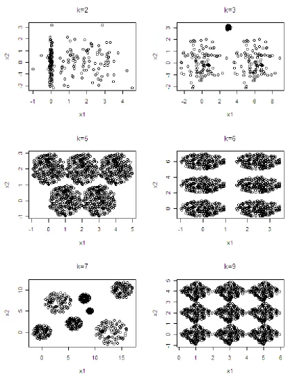
Initially, six two dimensional datasets are generated to be examined. Figure 5.1 contains the plot

(35)

[image:35.612.91.505.105.642.2]

(36)

The first example contains two clusters of 100 data points each, sampled from standard normal

distribution, with different mean and standard deviation.

The second simulated example contains three clusters of 100 points each. Two of the clusters

are of equal size and density and the third cluster in halfway between the first two, it is smaller and

more compact.

The third two dimensional example contains five spherical clusters of equal size and density,

some clusters slightly overlap.

Example four has six clusters of 200 points each, well separated spherical clusters.

The fifth example is made of seven well separated clusters of varying size and density,

contain-ing a total of 1400 data points.

The last example contains nine square clusters connected at the corners.

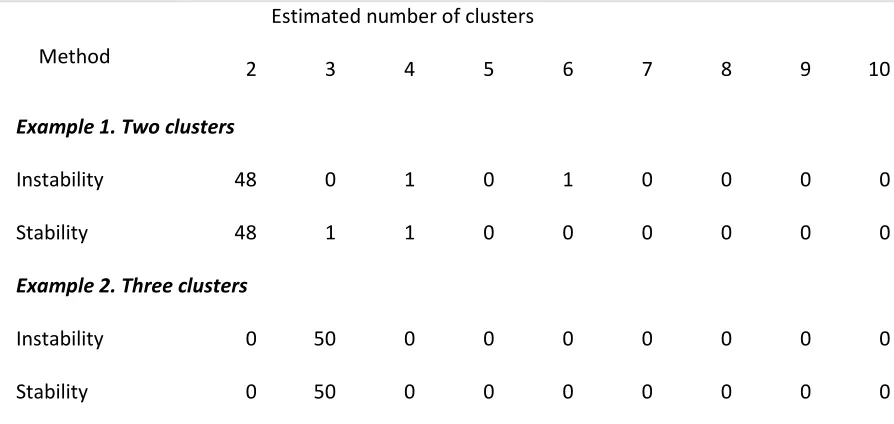
Each simulated example is repeated 50 times and the results are summarized in Table 5.1. Cross

validation with voting is used in both cases, and the k-means algorithm. Both stability and instability

yield superior performances in well-separated clusters (see Example 2 and 4). For the other examples

apparently both clustering algorithms tend to suggest far few clusters because the cluster separation

was not great enough for it to consider the clusters to be distinct. Example 6 is great to take in

consid-eration. Instability performs well every single time, in comparison to Stability which does it about 60% of

the time. The other 40% of the times it finds only one big cluster. Taking in consideration that the nine

squares are touching and that the whole graph is perfectly symmetrical it would probably make sense.

Stability performs far superior in Example 1, because the clustering stability measure is based on

(37)

[image:37.612.100.547.104.316.2]

Table 5.1. Two-dimensional examples: the estimated numbers of clusters using stability and instability

Method

Estimated number of clusters

2 3 4 5 6 7 8 9 10

Example 1. Two clusters

Instability 48 0 1 0 1 0 0 0 0

Stability 48 1 1 0 0 0 0 0 0

Example 2. Three clusters

Instability 0 50 0 0 0 0 0 0 0

Stability 0 50 0 0 0 0 0 0 0

Example 3. Five spherical clusters of equal size and density. Some clusters slightly overlap

Instability 23 0 0 27 0 0 0 0 0

Stability 50 0 0 0 0 0 0 0 0

Example 4. Six spherical clusters of equal size and density

Instability 0 0 0 0 50 0 0 0 0

Stability 0 0 0 0 50 0 0 0 0

Example 5. Seven well separated clusters of varying size and density

Instability 0 0 0 0 4 46 0 0 0

Stability 0 0 0 1 7 42 0 0 0

Example 6. Nine square clusters connected at the corners

Instability 0 0 0 0 0 0 0 50 0

(38)

[image:38.612.82.548.117.339.2]

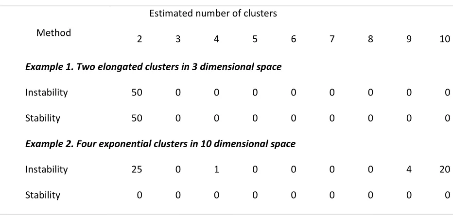
Table 5.2. Multi-dimensional examples: the estimated numbers of clusters using stability and

insta-bility

Method

Estimated number of clusters

2 3 4 5 6 7 8 9 10

Example 1. Two elongated clusters in 3 dimensional space

Instability 50 0 0 0 0 0 0 0 0

Stability 50 0 0 0 0 0 0 0 0

Example 2. Four exponential clusters in 10 dimensional space

Instability 25 0 1 0 0 0 0 4 20

Stability 0 0 0 0 0 0 0 0 0

Example 3 is another interesting one. Before we analyze the performance of the two methods

we should point out that clustering analysis does not offer an exact definition for the true k. As

men-tioned above some of the five spherical clusters overlap forming two bigger clusters. So, we can

con-clude that both stability and instability yield superior performances.

5.2.2 Multi-dimensional examples

To compare the performance of the two methods in question we are now going to examine two

multidimensional distance-based examples also found in Wang’s paper.

The first multi-dimensional dataset is Example 7, which is the same as the two elongated

clus-ters in three dimensions example in Tibshirani, Walther and Hastie (2001). The first cluster is generated

by taking 100 equally spaced values from -0.5 to 0.5 and Gaussian noise with standard deviation 0.1 is

(39)

[image:39.612.82.507.94.265.2]

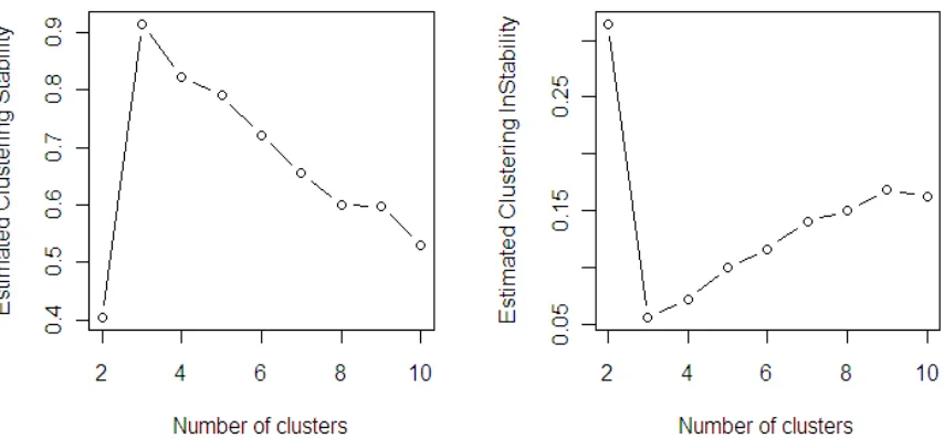
Figure 5.2 Estimated clustering stability and instability for Example 8 (four exponential clusters in 10 dimensional space)

added to each feature. As a result two elongated cluster are created, stretching out along the main

di-agonal of a three dimensional cube.

The eighth example contains four non-Gaussian clusters in a 10-dimensional space. Each cluster

is of size 100 and is sampled from standard exponential distribution centered at

( )

4, 4

,

(

4, 4

−

)

,

(

−

4, 4

)

and

(

− −

4, 4

)

; and the rest eight dimensions are noises sampled from standard exponential distribution.

Each simulated example is repeated 50 times, and the results are summarized in Table 5.2.

Both the stability and instability yield superior performances in Example 7, a low dimensional

example. As the dimension becomes high the two performs less satisfactory. Another reason behind the

performance could be that we are dealing here with non-Gaussian clusters. It is worth pointing out that

cross-validation with voting and k-means is used is both cases, which might not be the best option in this

(40)

[image:40.612.86.513.116.314.2]

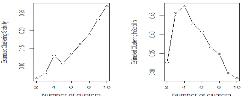
Figure 5.3 Estimated clustering stability and instability for the wine data

5.3 Real Examples

We now examine the effectiveness of the new defined stability on two real life examples.

The first example is the iris data (Fisher, 1936), which is perhaps the best known database in

pattern recognition literature. The dataset contains 150 observations from three different species of iris

(Setora, Versicolour, Virginica), each with four attributes: length and width of sepal, length and width of

petal.

The second real life example is the wine data set (Forina, M. et al, PARVUS), which contains

re-sults of a chemical analysis of wines grown in Italy and derived from three different cultivars. The 178

data points consist of 12 measurements.

The true value of k is usually unknown when real data is examined. The iris data contains three

species of iris so we would estimate the number of clusters for this data set to be three. Likewise

(41)

k. The estimated clustering stability and instability curves for the iris data are both summarized in Figure

1.1. The clustering stability achieves its highest value atkɵ=2, result that is acceptable for clustering as it

is known that two of the species are undistinguishable (Sugar & James, 2003). The estimated clustering

stability and instability curves for the wine data are displayed in Figure 5.3. The clustering stability curve

(42)

CHAPTER 6

Discussion

In this thesis, we propose some novel criteria for selecting the number of clusters that are

appli-cable to various clustering algorithm. The previous proposed approaches are focusing on maximizing the

within-cluster similarity and/or within cluster dissimilarity. Wang’s proposed selection criteria measure

the quality of clustering through instability from sample to sample. The proposed selection criteria

measure the quality of clustering through stability from sample to sample. This stability measure is

as-sumption free and applicable to both distance based and non-distance based clustering algorithms; and

it is measured by the correlation between two clustering functions. Modified cross validation schemes

are used, which are more reliable when there is no compelling evidence to justify the model

assump-tion.

We should point out that determining the real number of clusters is a major challenge of

clus-tering analysis. Unfortunately, the true number of clusters is not a well defined concept in the statistical

literature. The proposed criterion is one of the many practical ways of defining the true number of

clus-ters. Due to the lack of objective definition of a proper clustering, deciding which method is the best is

almost an impossible task. We can only claim that clustering stability can be useful criterion for

assess-ing the goodness of clusterassess-ing algorithms.

The advantages and disadvantages of the proposed criteria are demonstrated, both numerically

(43)

REFERENCES

Akaike, H. (1974). A new look at the statistical model identification. IEEE Transactions on Automatic

Con-trol 19 (6): 716–723.

Baxter, R. A. & J. J. Oliver. The Kindest Cut: Minimum Message Length Segmentation. In Alg rithmic

Learning Theory, 7th Intl. Workshop, 83-90. Sydney, Australia, 1996.

Ben-David, S., Von Luxburg, U. & Pal, D. (2006). A sober look at stability of clustering. In Proc. 19th Ann.

Conf. Learn. Theory (COLT 2006), Ed. G. Lugosi and H. Simon, pp. 5–19. Berlin: Springer.

Ben-Hur, A., Elisseeff, A. & Guyon, I. (2002). A stability based method for discovering structure in

clus-tered data. In Pac. Symp. Biocomp. 2002, 6–17.

Burman, P. (1989).Acomparative study of ordinary cross validation, v-fold cross validation and the

re-peated learningtesting methods. Biometrika 76, 503–14.

Calinski, R. B. & Harabasz, J. (1974). A dendrite method for cluster analysis. Commun. Statist. 3, 1–27.

Dubes RC. How many clusters are best?—An experiment. Pattern Recognition 1987; 20: 645-663.

Forina, M. et al, PARVUS - An Extendible Package for Data Exploration, Classification and Correlation.

Institute of Pharmaceutical and Food Analysis and Technologies, Via Brigata Salerno, 16147

Ge-noa, Italy.

Fang, Y. & Wang, J.(2011). Penalized cluster analysis with applications to family data. CSDA, 55,

2128-2136.

Fraley, C. & E. Raftery. How many clusters? Which clustering method? Answers via model-based Cluster

Analysis. In Computer Journal, vol. 41, pp. 578-588, 1998.

Geisser, S. (1975). The predictive sample reuse method with applications. J. Am. Statist. Assoc. 70, 320–

8.

Hansen, M. & B. Yu. Model Selection and the Principle of Minimum Description Length. In JASA, vol. 96,

(44)

Hartigan, J. A. (1975). Clustering Algorithms. New York: Wiley.

Janson, S. (2004). Large deviations for sums of partly dependent random variables. Random Struct.

Al-gor. 24, 234–48.

Kaufman, L. & Rousseeuw, P. (1990). Finding Groups in Data: An Introduction to Cluster Analysis. New

York: Wiley.

Krieger, A. M. & Grenn, P. E. (1999). A cautionary note on using internal cross validation to select the

number of clusters. Psychometrika 64, 341–53.

Krzanowski, W. J. & Lai, Y. T. (1985). A criterion for determining the number of clusters in a data set.

Biometrics 44, 23–34.

Lange, T., Roth, V., Braun, M. & Buhmann, J. (2004). Stability-based validation of clustering solutions.

NeuralComp. 16, 1299–323.

MacQueen, J. B. (1967). "Some Methods for classification and Analysis of Multivariate Observations,

Proceedings of 5th Berkeley Symposium on Mathematical Statistics and Probability”, University

of California Press. pp. 281–297.

Milligan GW, Cooper MC. An examination of procedures for determining the number of clusters in a

da-ta set. Psychometrika 1985; 50: 159–179.

Mccullagh, P. & Yang, J. (2008). How many clusters? Bayesian Anal. 3, 101–20.

NG, A., Jordan, M. & Weiss, Y. (2001). On spectral clustering: analysis and an algorithm. In Adv. Neural.

Info. Processing Sys. (NIPS2001), Ed. T. Dietterich, S. Becker and Z. Ghahramani, pp. 849–56.

Cambridge:MIT Press.

Pedrycz, W. (2005). Interpretation of clusters in the framework of shadowed sets. Pat. Recog. Lett. 26,

2439–49.

(45)

Rissanen, J. Fisher information and stochastic complexity, IEEE Transactions on Information Theory, vol.

IT-42, 1, pp. 40–47, 1996.

Rissanen, J. Complexity and information in data. In Proc. IFAC Conf. System Identification, SYSID 2000,

Santa Barbara, CA, 200

Roth, V., T. Lange, M. Braun & J. Buhmann. A Resampling Approach to Cluster Validation. In Intl. Conf. on

Computational Statistics, pp. 123-129, 2002.

Salvador, S. & Chan, P., Determining the Number of Clusters/Segments in Hierarchical

Cluster-ing/Segment Algorithms, ICTAI 2004, pp. 576-584

Schwarz, G. (1978). Estimating the dimension of a mode, The Annas of Statistics, 6, 461-464

Shamir, O. & Tishby, T. (2007). Cluster stability for finite samples. In Adv. Neural Info. Processing Sys.

(NIPS2007),Ed. J. Platt, D. Koller, Y. Singer and S. Roweis, pp. 1297–304. Cambridge: MIT Press.

Shao, J. (1993). Linear model selection by cross validation. J. Am. Statist. Assoc. 88, 486–94.

Shi, J. & Malik, J. (1997). Normalized Cuts and Image Segmentation, Proc. IEEE Conf. Computer Vision

and Pattern Recognition, pp. 731-737.

Smyth, P. Clustering using Monte Carlo cross validation. In Proc. 2nd Intl. Conf. Knowl. Discovery & Data

Mining (KDD-96), Portland, OR, 1996; 126–133.

Smyth, P. Clustering Using Monte-Carlo Cross Validation. In Proc. 2nd KDD, pp.126-133, 1996.

Steinhaus, H. (1956). "Sur la division des corps matériels en parties" (in French). Bull. Acad. Polon. Sci. 4

(12): 801–804.

Sugar , C. & James, G. (2003). Finding the number of clusters in a data set: an information theoretic

ap-proach. J. Am.Statist. Assoc. 98, 750–63.

Sugiyama, M. & H. Ogawa. Subspace Information Criterion for Model Selection. In Neural Computation,

(46)

Tibshirani, R., Walther, G.,Botstein, D. & Brown, P. (2001a). Cluster validation by prediction strength. J.

Comp.Graph. Statist. 14, 511–528.

Tibshirani, R., Walther, G. & Hastie, T. (2001b). Estimating the number of clusters in a data set via the

gap statistic. J. R. Statist. Soc. B 63, 411–23.

Von Luxburg, U., Belkin, M. & Bousquet, O. (2008). Consistency of spectral clustering. Ann. Statist. 36,

555–86.

Wang, J. (2010). Consistent selection of the number of clusters via cross-validation. Biometrika, 97,

893-904.

Yang, Y. (2006). Comparing learning methods for classification. Statist. Sinica 16, 635–57.

Yang, Y. (2007). Consistency of cross validation for comparing regression procedures. Ann. Statist. 35,

2450–73.

(47)

APPENDICES

Appendix A: R code for simulation

#################################################### # MAIN FUNCTIONS

#################################################### #

# Stability and Instability Curves - 2 Dimensional Data #

#################################################### ####################################################

##################### 2 clusters ######################

stab.avg=rep(0,10) # simulation results instab.avg=rep(0,10) # simulation results stab=matrix(NA, 50, 10) # instability matrix instab=matrix(NA, 50, 10) # instability matrix

for (k in 2:10) {

for (i in 1:50)

{ sim2=matrix(0,200,2) x1=rnorm(100,0,1) x2=rnorm(100,0,1) sim2[,1]=c(.05*x1,x1+3) sim2[,2]=c(x2,x2) data.sd=stand(sim2)

instab[i,k]=clus.cv(data.sd,k) # instability measure given k stab[i,k]=clus.cv.new(data.sd,k) # stability measure given k }

stab.avg[k]<-mean(stab[,k]) instab.avg[k]<-mean(instab[,k]) }

################## 3 clusters ##################