https://doi.org/10.5194/hess-21-5971-2017 © Author(s) 2017. This work is distributed under the Creative Commons Attribution 3.0 License.
On the value of water quality data and informative flow states
in karst modelling
Andreas Hartmann1,2, Juan Antonio Barberá3, and Bartolomé Andreo3
1Faculty of Environment and Natural Resources, University of Freiburg, Freiburg, Germany 2Department of Civil Engineering, University of Bristol, Bristol, UK
3Department of Geology and Centre of Hydrogeology, University of Malaga (CEHIUMA), Malaga 29071, Spain
Correspondence to:Andreas Hartmann ([email protected]) Received: 18 April 2017 – Discussion started: 10 May 2017
Revised: 11 October 2017 – Accepted: 12 October 2017 – Published: 30 November 2017
Abstract.If properly applied, karst hydrological models are a valuable tool for karst water resource management. If they are able to reproduce the relevant flow and storage processes of a karst system, they can be used for prediction of water resource availability when climate or land use are expected to change. A common challenge to apply karst simulation models is the limited availability of observations to identify their model parameters. In this study, we quantify the value of information when water quality data (NO−3 and SO2−4 )is used in addition to discharge observations to estimate the pa-rameters of a process-based karst simulation model at a test site in southern Spain. We use a three-step procedure to (1) confine an initial sample of 500 000 model parameter sets by discharge and water quality observations, (2) identify alter-ations of model parameter distributions through the confine-ment, and (3) quantify the strength of the confinement for the model parameters. We repeat this procedure for flow states, for which the system discharge is controlled by the unsatu-rated zone, the satuunsatu-rated zone, and the entire time period in-cluding times when the spring is influenced by a nearby river. Our results indicate that NO−3 provides the most information to identify the model parameters controlling soil and epikarst dynamics during the unsaturated flow state. During the sat-urated flow state, SO2−4 and discharge observations provide the best information to identify the model parameters related to groundwater processes. We found reduced parameter iden-tifiability when the entire time period is used as the river in-fluence disturbs parameter estimation. We finally show that most reliable simulations are obtained when a combination of discharge and water quality date is used for the combined unsaturated and saturated flow states.
1 Introduction
It is estimated that around 10–15 % of emerged Earth surface is covered by soluble rocks that are susceptible to be karsti-fied (Ford and Williams, 2007). Today, aquifers developed in such types of rock roughly supply groundwater to a quarter of the world’s population. The importance of groundwater resources from karst aquifers is not only limited to satisfy the fresh water demand of large regions with millions of in-habitants (e.g. Austria or Slovenia) but also it guarantees the water supply in small settlements where karst waters are the only source of drinking water.
that the unsaturated zone, jointly with soil and epikarst, acts chemically as a reaction layer that is able to modify the groundwater quality in a substantial way.
Simulation models are a common tool to address water management questions such as the impacts of climate and land use changes on karst water resources (Hartmann et al., 2014a). In order to provide reliable predictions, these models need to include the most relevant processes of karst systems and various approaches have been developed to include karst processes in distributed and lumped karst simulation models (Ghasemizadeh et al., 2012; Hartmann et al., 2014a; Hart-mann and Baker, 2017; Kovacs and Sauter, 2007; Sauter et al., 2006). The choice of the model approach is usually due to the required purpose. A key challenge in all of these karst modelling approaches is the identification of the model pa-rameters. Methods to explore and analyse karst systems can provide prior knowledge on karst system properties (Gold-scheider and Drew, 2007) that can be used to gain prior in-formation on karst model parameters such as hydraulic con-ductivities or catchment boundaries. However, capturing the entire heterogeneity of karst systems with those methods is commonly impossible (Hartmann et al., 2013a) and inverse parameter estimation schemes, for instance automatic cali-bration by observed discharge, have to be applied.
Work with automatic calibration approaches showed that using only discharge observations for model calibration al-lows us to identify up to six model parameters (Jakeman and Hornberger, 1993; Wheater et al., 1986; Ye et al., 1997). More recent works also revealed that including disinforma-tive periods in the calibration, i.e. periods when errors in the observation can be expected, may significantly bias the results of model calibration and evaluation of hydrological models (Beven et al., 2011; Beven and Westerberg, 2011; Kauffeldt et al., 2013). Due to the complexity of karst pro-cesses, karst models usually require more than six model parameters to reflect the most important hydrological pro-cesses. Some studies tried to compensate for this apparent lack of information by using auxiliary data such as gravimet-ric information (Mazzilli et al., 2012), artificial tracer exper-iments (Hartmann et al., 2012; Oehlmann et al., 2015), or hydrochemical information (Charlier et al., 2012; Hartmann et al., 2013b, 2016). However, to our knowledge the problem of disinformative observations, either discharge observations or auxiliary information, has not been addressed explicitly in karst modelling studies.
This study proposes a new approach to quantitatively as-sess the information content of discharge and hydrochemi-cal information for karst model hydrochemi-calibration including periods with disinformative observations. A process-based model is used to simulate the hydrodynamic and hydrochemical (NO−3 and SO2−4 )behaviour of a karst system, at which the unsat-urated zone dynamics dominate under recharge conditions, controlling groundwater flow and solute transport processes. During specific periods, the discharge and chemistry of the
system is influenced by the surface flow of a nearby river, which constitutes disinformative periods for model parame-ter estimation. A new parameparame-ter estimation approach is em-ployed to estimate the information content of the different types of calibration data during predefined flow states that focus on time periods dominated by unsaturated zone dis-charge, saturated zone disdis-charge, and periods that include the disinformative observations. Even though it is applied to only one particular study site this approach can easily be trans-ferred to any hydrological system where different observa-tion types are available for calibraobserva-tion.
2 Study site description
The experimental area is located in the eastern Ronda moun-tains, in the NW of Málaga province (southern Spain). It con-sists of steep and rugged NE–SW oriented reliefs (e.g. Sierra Blanquilla), reaching a maximum height of 1 428 m a.s.l. (Viento peak; Fig. 1). Geologically, three main stratigraphic groups can be differentiated (Cruz-Sanjulián, 1974; Martín-Algarra, 1987; Fig. 1): (i) clays and evaporites of upper Tri-assic age (the older formation), (ii) a thick (up to 500 m) carbonate sequence of Jurassic dolostones and limestones forming the main aquifer (i.e. Sierra Blanquilla), and (iii) Cretaceous-Paleogene marls and marly limestones as the up-permost materials. The geological structure of the Sierra Blanquilla is constituted by a NE–SW oriented box-shaped anticline, plunging towards NE (Martín-Algarra, 1987), with a flat and wide hinge, as well as subvertical flanks. The folded structure is also fractured by two sets of faults 50◦N–70◦E
and N150E oriented (Fernández, 1980). From the point of view of the karst landscape development in plateau areas, the horizontal bedding planes of carbonate exposures together with the high precipitation rate have favoured the formation of exokarstic features including karrenfields, dolines, uvalas, shafts, and swallets, as a result of intense karstification pro-cesses.
2.1 Karst hydrogeology
Figure 1.Geographic, geological, and hydrogeological features of the Sierra Blanquilla carbonate aquifer.
located upstream of the permanent ones, activate after heavy rainfall events (Barberá and Andreo, 2015). Low flow is es-tablished when the permanent groundwater flow (from BG and HB springs) is below 0.2 m3s−1.
The main hydrological feature in the test site, the Turón river, intermittently crosses the carbonate exposures at the southern border of the Blanquilla aquifer (Fig. 1). The sur-face flow has been demonstrated to alter the hydrodynamic functioning of both perennial springs (Barberá and Andreo, 2015), which are partly affected by the existence of two regu-lation dams (20–25 m high) built over the Turón riverbed, just several tens of meters downstream from the springs (Fig. 1). In high-flow periods, both headwater and groundwater dis-charge from the Sierra Blanquilla aquifer maintain the river flow, while during low-flow conditions, the Turón river is ex-clusively fed by karst groundwater.
2.2 Dominant hydrogeological processes
Electrical conductivity (EC) has been used as a global physicochemical marker for distinguishing the hydrochem-ical states that characterize the El Burgo spring discharge. Generally, EC peaks seem to be concomitant with maximum spring discharge on the event scale, which is evidence that more mineralized groundwater is drained immediately after each rainfall episode (green shaded areas in Fig. 2). Barberá and Andreo (2015) stated that this high EC groundwater is also characterized by higher alkalinity and logPCO2 values
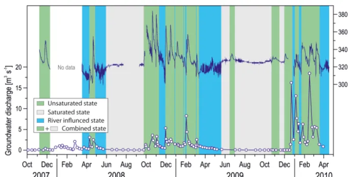
unsatu-Figure 2.Decomposition of the El Burgo spring flow in selected hydrochemical states from EC and discharge time series: (1) unsaturated zone dominates discharge; (2) saturated zone dominates discharge; and (3) discharge (and EC) influenced by the Turón river flow; the combination of unsaturated and saturated states represents the combined flow state.
rated and saturated zone until the discharge zone by a subse-quent recharge pulse. Therefore, unsaturated flow dominates under high-water conditions in the El Burgo spring (unsatu-rated state in Fig. 2).
Under low-flow conditions (no rainfall, light gray areas with data areas in Fig. 2), EC levels in the groundwater re-main quite stable in the range of 320–330 µS cm−1. This pro-vides the chemical baseline of the system (saturated state in Fig. 2), which is dependent on the accumulated rainfall on each hydrological year. The lower and less variable EC values of groundwater compared with those obtained un-der high-water conditions can be explained by the loss of “aggressiveness” of groundwater (degassed waters with re-spect to CO2)flowing through the system as a consequence
of the lack of aquifer recharge (Barberá and Andreo, 2015). Therefore, groundwater drainage under low-water conditions consists of a system of slower flows coming from capaci-tive compartments of the aquifer (the phreatic zone). With these circumstances, the functioning of the hydrogeologi-cal system is mainly dominated by the saturated zone (sat-urated state in Fig. 2). Even though there still might be some seepage from the soil and epikarst during this stage, the hy-drochemical signature of the spring, which is dominated by the signal of the phreatic zone (Barberá and Andreo, 2015), shows that these fractions are not very important.
Marked dilutions in groundwater mineralization (below the chemical baseline of the system), which very often oc-cur during the spring recession after flood events, are also observed in the chemograph of the El Burgo spring (pref-erentially from March to June in Fig. 2). Since the Turón river waters are less mineralized than groundwater and that the temporary storage of surface water in the nearby river dam favours water mixing, surface water dilutes groundwater from the spring (river influenced state in Fig. 2). This occurs
when the river stage is higher than the groundwater level in the discharge zone, promoting water flow towards the aquifer (Barberá and Andreo, 2015).
3 Methodology 3.1 Available data
Continuous daily measurements of precipitation and air tem-perature were recorded at Añoreta weather station (Fig. 1) and discrete sampling campaigns for meteoric water chem-istry (NO−3 and SO2−4 among others) were performed in a rain collector installed to the north of Viento peak (Fig. 1), from August 2007 to April 2010. From meteorological data, potential evapotranspiration was calculated on a daily time scale using Thornthwaite’s approach (Thornthwaite, 1948). Discontinuous measurements of the Turón river flow in two selected sections (TupandTdn), upstream and downstream of
[image:4.612.129.470.68.241.2]Table 1.Main characteristics of the time series of hydrodynamic and hydrochemical data used in this study. CV is the coefficient of variation.
Sampling site Parameter Unit n Max Min Mean CV Average sampling Period
(%) frequency
Añoreta weather st. rainfall (accumulated) mm day−1 959 71 0 3.3 – 1 day 16/08/2007–31/03/2010 air temperature (daily mean) ◦C 959 14.9 2.6 8 – 1 day 16/08/2007–31/03/2010
Viento rain collector NO−3 mg L−1 38 23 0 3 2 15 days∗ 04/10/2007–16/02/2010
SO24− mg L−1 38 4.9 0.3 1.2 1 15 days∗ 04/10/2007–16/02/2010
Turón river discharge (GW component) m3s−1 132 18.5 0.06 1.63 169 7 days 16/08/2007–30/03/2010 El Burgo spring electrical conductivity (EC) µS cm−1 17 296 384 288 326 3 1 h 07/11/2007–15/04/2010
NO−3 mg L−1 130 21.2 0.8 5.1 56 8 days 01/08/2007–30/03/2010
SO24− mg L−1 130 24.4 4.2 11.4 49 8 days 01/08/2007–30/03/2010
∗Sampling frequency was dependent on the occurrence of rainfall episodes.
states of the system (Sect. 2.2) was used to provide an inde-pendent consideration of observations that can be attributed to time periods of the unsaturated state, saturated state, and all states including the period influenced by the Turón river dynamics (river influenced state).
3.2 The model
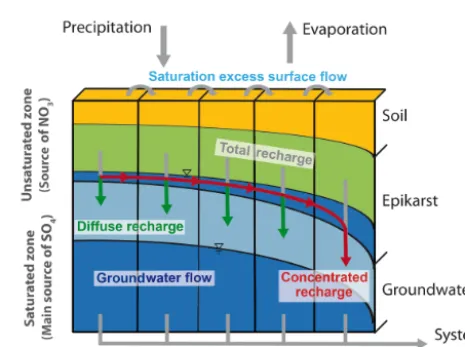
The VarKarst model was previously developed at a neigh-bouring karst system in southern Spain (Hartmann et al., 2013b) and it was successfully applied at different karst sys-tems around Europe (Brenner et al., 2016; Hartmann et al., 2013a, 2014b, 2016). It includes the variability of karst sys-tem properties by statistical distribution functions (Fig. 3). Explicitly, it considers the spatial variability in (i) soil and epikarst depths, (ii) fractions of concentrated and diffuse recharge to the groundwater, (iii) epikarst hydrodynamics, and (iv) groundwater hydrodynamics by distribution func-tions that are applied to a set of N model compartments. This allows the simulation of variably dynamic pathways of water and solutes through the karst system. Solute transport simulations within the model follow the assumption of in-stantaneous and complete mixing within each storage (soil, epikarst, groundwater) and each of the N model compart-ments (Fig. 3). In the particular case of NO−3, this implies neglecting plant uptake and release processes, which were found to be important in more humid regions (Hartmann et al., 2016) but it was found a valid assumption at Mediter-ranean regions such as our study site (Hartmann et al., 2013b, 2014b). The detailed equations of the model are in the ap-pendix and a list of all model parameters including their de-scription are provided in Table 2.
3.3 Parameter estimation for the distinctive flow states and different observation types
The low resolution of observed discharge and hydrochem-istry as well as the complex karstic setting of the study site creates a rather uncertain environment for modelling. For that reason, a traditional multi-objective parameter es-timation was omitted as in previous studies (Hartmann et al., 2013b, 2016). Instead, a parameter estimation scheme
Figure 3.Schematic representation of the VarKarst model structure (modified from Hartmann et al., 2013a).
considering “soft rules” was used to confine a large uni-formly sampled set of model parameters therefore explicitly allowing for some uncertainty to remain but to be quanti-fied. A similar approach was already applied successfully in the frame of a large-scale karst groundwater recharge study (Hartmann et al., 2015, 2017).
As a measure of performance, the Kling–Gupta efficiency KGE (Gupta et al., 2009) is used. It is defined to show num-bers approaching 1 for the best simulations:
KGE=1− q
(r−1)2+(α−1)2+(β−1)2, (1)
with
α= σS σO
andβ= µS µO
. (2)
rexpresses the linear correlation coefficient between simula-tions and observasimula-tions, whileµS/µOandσS/σOare defined
[image:5.612.311.544.230.404.2]time steps for which observations are available are consid-ered. Hence, the KGE values will only express the model performance to reflect the discharge, NO−3, and SO2−4 obser-vations that were sampled in a 7- to 8-day temporal resolu-tion (Table 1) even though the model runs on a daily time step.
For parameter estimation, an initial sample of 500 000 parameter sets was created from predefined ranges (Ta-ble 2) that were chosen by prior knowledge and previous model experiences in the same region (Hartmann et al., 2013b, 2014b). A 4-year warm-up period was set up and the model was run 500 000 times with the initial parame-ter sample. Using the observed time series, the Kling–Gupta efficiency was calculated for each of the simulation runs: KGEQ(groundwater discharge), KGENO3 (NO
−
3
concentra-tions) and KGESO4 (SO
2−
4 concentrations). Similar to Choi
and Beven (2007) “soft rules” were used to reduce the initial sample of parameters in four steps:
– All parameter sets from the initial sample with KGEQ<0.2 were discarded.
– All parameter sets from the initial sample with KGENO3<0.2 were discarded.
– All parameter sets from the initial sample with KGESO4<0.2 were discarded.
– All parameter sets from the initial sample with KGEQ, KGENO3, and KGESO4<0.2 at the same time were
dis-carded.
The threshold value of 0.2 was found by preliminary anal-ysis. Its rather low value is meant to take into account that the simulation is exposed to various sources of uncer-tainty including uncertainties in the model input (observa-tion of climate variables and their applica(observa-tion to the entire recharge area), model structure uncertainty (representation of karst processes by conceptual mathematical formulations in a semi-distributed way), and the uncertainty of observations (discharge measurement and hydrochemical analysis, as well as their low temporal resolution).
The application of the soft rules is repeated four times for observations falling into the unsaturated flow state, the satu-rated flow state, the combined unsatusatu-rated and satusatu-rated flow state and into the entire time period including the hydrody-namic state defined by the influence of the Turón river flow on groundwater discharge. For each of these time periods the four soft rules will result in a reduction in the initial sample, and the prior ranges of the model parameters will experience a confinement (Hartmann et al., 2015).
3.4 Evaluation of information content and simulation uncertainty for the different flow states and different observation types
In this study, the strength of this confinement is used to as-sess the information content of the set of observations during
the different flow states. The strength of the confinement is quantified by the reduction in the distance between the 25th and 75th percentiles of each model parameter after the con-finement through the soft rules. For instance, parametercSO4
(Table 2) has the prior range of 0–100 mg L−1. Consequently, the uniform sampling strategy for the initial sample will re-sult in values close to 25 and 75 mg L−1for the 25th and 75th percentiles, respectively. Applying one of the soft rules may now result in values of 10 and 30 mg L−1 for the 25th and 75th percentiles, respectively. Hence, the reduction in the dis-tance between the 25th and 75th percentiles is 50–20 mg L−1, i.e. a reduction of 60 % took place. In this example case, we would find that the observations applied through the selected soft rule provided useful information to estimate this parame-ter. Applying this procedure for each of the four soft rules and the four time series defined by the flow states, we can assess how (1) the different types of observations (discharge, NO−3 and SO2−4 )contribute to parameter identification, and (2) the focus on particular time periods and flow stages strengthens or weakens the confinement of the model parameters.
Particular attention is given to the comparison of the en-tire time period, including the times when the spring is influ-enced by the river, with the time periods when only the un-saturated zone and the un-saturated zone control the discharge of the spring. It is expected that this time period contains disinformative information for parameter estimation as the VarKarst model does not take into account the river’s influ-ence. The reduction between the 25th and 75th percentiles of the model parameters is used after applying the fourth soft rule (Sect. 3.3) of the combined unsaturated and saturated flow state, and the entire time period including the period that is influenced by the river to understand the impact of the disinformative information on parameter identification. In a last step, the simulation uncertainty is quantified for the two time periods by plotting the simulations of the parameter sets that remained after the fourth soft rule was applied to the two observation time series. After including the disinformative time period, a greater simulation uncertainty is expected.
4 Results
4.1 Parameter estimation for the different flow states and different observation types
Different reductions of the initial sample are found by the dif-ferent soft rules and during the difdif-ferent flow states (Fig. 4). The reduction by discharge (KGEQ≥0.2) varies among the different flow states but remains rather limited. The same is seen for the individual use of the hydrochemical information (KGENO3≥0.2 or KGESO4≥0.2). However, using the
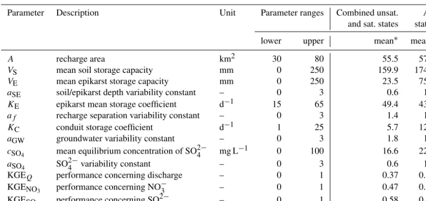
Table 2.Description of model parameters, ranges for parameters estimation and average values found for the combined unsaturated and saturated flow states, and the entire time period including the disinformative period of river influence.
Parameter Description Unit Parameter ranges Combined unsat. All and sat. states states
lower upper mean∗ mean∗
A recharge area km2 30 80 55.5 57.5
VS mean soil storage capacity mm 0 250 159.9 174.1 VE mean epikarst storage capacity mm 0 250 23.5 75.8 aSE soil/epikarst depth variability constant – 0 3 0.6 1.8 KE epikarst mean storage coefficient d−1 15 65 49.4 43.4 af recharge separation variability constant – 0 3 1.4 1.3 KC conduit storage coefficient d−1 1 25 5.7 12.4 aGW groundwater variability constant – 0 3 1.8 1.3 cSO4 mean equilibrium concentration of SO
2−
4 mg L−1 0 100 16.6 22.0
aSO4 SO
2−
4 variability constant – 0 3 0.6 1.4
KGEQ performance concerning discharge – 0 1 0.37 0.36 KGENO3 performance concerning NO
−
3 – 0 1 0.47 0.32
KGESO4 performance concerning SO
2−
4 – 0 1 0.58 0.40
∗variability of model parameters shown in Fig. 5.
Figure 4.Reduction in the initial sample by the four soft rules for the unsaturated state, saturated state, combined saturated and satu-rated states, and all system states.
rules is found for the consideration of all stages including the disinformative time period influenced by the river.
The influence of the soft rules during the different flow states varies for all model parameters (Fig. 5). The reduc-tion in the initial sample by discharge (KGEQ≥0.2) alters the uniform distribution of the initial sample for the different flow states, mostly for the parametersA,VE, andKC. These
changes are most prominent in the unsaturated state (A), the saturated state (VEandKC), and the combined unsaturated
and saturated states (A,VE, and KC). Using NO−3 for the
reduction (KGENO3≥0.2), the parametersVS,VE, andaSE
experience the strongest change in their initial distribution. This change is most pronounced at the unsaturated state and
the combined unsaturated and saturated states. The reduction by the observations of SO2−4 concentrations (KGESO4≥0.2)
mostly affects the model parameterscSO4 andaSO4, but also
find a strong impact onaSE, mainly at the saturated state and
the combined unsaturated and saturated state. Finally apply-ing all information in the fourth soft rule (all KGE≥0.2), we find again an alteration of the model parameters that were af-fected by soft rules 1–3 (A,VE,VS,aSE,KC,cSO4, andaSO4)
and, additionally, a moderate alteration ofVE andaf. This is most notable at the combined unsaturated and saturated states; using all states including the disinformative period that is influenced by the river the alterations are generally less pronounced.
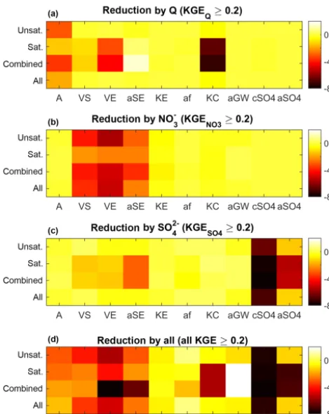
4.2 Evaluation of information content and simulation uncertainty for the distinctive flow states and different observation types
Using the change in distance between the 25th and 75th percentiles of each model parameter for the different soft rules and the different flow states we are able to quantify the information content of the available observations (Fig. 6). We find that discharge (KGEQ≥0.2) and SO2−4 (KGESO4≥
0.2) provide most information during the saturated flow state, while NO−3 reduces the distance between the two percentiles most during the unsaturated stage. The state that uses all in-formation including the disinformative time period of river influence shows generally the weakest reduction between the 25th and 75th percentiles as already indicated by Fig. 4.
[image:7.612.50.285.334.494.2]Figure 5.Distribution of model parameters (normalized by their ranges) after applying the four soft rules for the unsaturated, saturated, combined unsaturated and saturated, and all stages.
provides the most information on the parameterKC, but the
change in distance for the parametersAandVEis still
con-siderable. This is most evident in the combined unsaturated and saturated states. We find a more balanced distribution of information on the altered parameters when regarding the re-duction obtained by NO−3 (KGENO3≥0.2). Here, the change
in distances is considerable (but similar) for VS, VE, and
aSE. For SO2−4 (KGESO4 ≥0.2), the alteration mostly affects
cSO4, followed by a considerable alteration in aSO4 and a
moderate change inaSE. Using all information to confine the
initial sample (all KGE≥0.2) shows that the combined use of discharge, NO−3 and SO2−4 observations provide the most information on VE,aSE,KC,cSO4, and aSO4. Still,
consid-erable information is provided forA,VS, andaf. However, no reduction in the distance between the 25th and 75th per-centiles is found forVE, and even a widening takes place for
aGW.
The proceeding analysis indicates that most information to identify the largest number of model parameters is pro-vided by the combined unsaturated and saturated flow states using discharge, NO−3, and SO2−4 observations. It further re-veals that using the entire time period, using discharge, NO−3,
and SO2−4 observations and including the period that is influ-enced by the river, provided the least information; only 5 (A,
VS,VE,aSE, andcSO4)of the 10 model parameters show a
detectable reduction in the two flow percentiles (Fig. 6, bot-tom).
The final averages of the estimated parameters (after ap-plying the 4th soft rule; Table 2) of the combined unsaturated and saturated flow states, and the state that uses the entire set of observations are similar for the parametersA,VS, and
cSO4, while there is a strong difference forVEandaSE.
Figure 6.Change in distance between the 25th and 75th percentiles of each model parameter when the different soft rules are applied (top to bottom) for the four flow states.
5 Discussion
5.1 Application of the soft rules during the different flow states
The application of the four soft rules results in a general re-duction in the initial sample for all flow states (Fig. 4). A weak reduction for all four flow states takes place when only discharge observations are applied to confine the sample. Previous research with lumped model calibration showed that the information content of discharge observations usu-ally suffices to calibrate 5–6 parameters (Jakeman and Horn-berger, 1993; Wheater et al., 1986; Ye et al., 1997); more parameters often lead to over parameterization (Perrin et al., 2003) and equifinality (Beven, 2006). Hence, the small re-duction in the VarKarst initial parameter sample may be due to the large number of model parameters (Table 2) within the VarKarst model. The same behaviour of a weak decrease in the initial parameter sample is found when the hydro-chemical observations are used individually (soft rules 2 and 3). The weakest reduction in the initial parameter sample among all four flow states is found for the entire time period that includes the periods of river influence (see discussion in Sect. 5.2).
When soft rule 4 (all KGE≥0.2) is applied, we find the strongest reduction in the initial sample across all of the four flow states. This means that the combined information of discharge, NO−3, and SO2−4 observations provides the most information to reduce the initial sample of model parame-ters. Previous research already showed that hydrochemical information can reduce parameter uncertainty (Kuczera and Mroczkowski, 1998; Rimmer and Hartmann, 2014; Son and Sivapalan, 2007). In this study, a similar reduction in param-eter uncertainty could be observed (Fig. 5). Depending on the applied soft rule and the considered flow states, the initially uniform distributions of the model parameters are altered dif-ferently. Some model parameter distributions change their mean without much change in the shape of their distribution (same distance between 25th and 75th percentiles); some of them show a more confined distribution when the soft rules are applied.
5.2 Information provided by discharge and hydrochemistry during the different flow states The differences in the reduction across the model parame-ters reveals the influence of different types of observations that were used for parameter estimation. We find that the reductions of the distance between the 25th and 75th per-centiles is most pronounced during the saturated stage for the discharge observations (Fig. 6). This indicates that dis-charge provides the most information during the recession period. Information about hydrodynamic parametersA,VE,
andKCis derived directly from the discharge observations.
This makes sense because hydrodynamic changes in the main discharge area of the Sierra Blanquilla aquifer reflect the hy-draulic pressure transference from the unsaturated zone to the saturated zone of the system. Similar results were found by Wagener et al. (2003) when they applied dynamic identifi-ability analysis to a lumped rainfall-runoff model using only discharge data.
They also found that the parameters, which control the unsaturated zone and fast flow components of their model, are most identifiable during and just after the rainfall-runoff events. Our results indicate a similar behaviour by show-ing the strongest reduction in the distance between the 25th and 75th percentiles for the unsaturated zone parameters dur-ing the unsaturated flow state usdur-ing the NO−3 observations (parametersVS, VE, and aSE). This is in accordance with
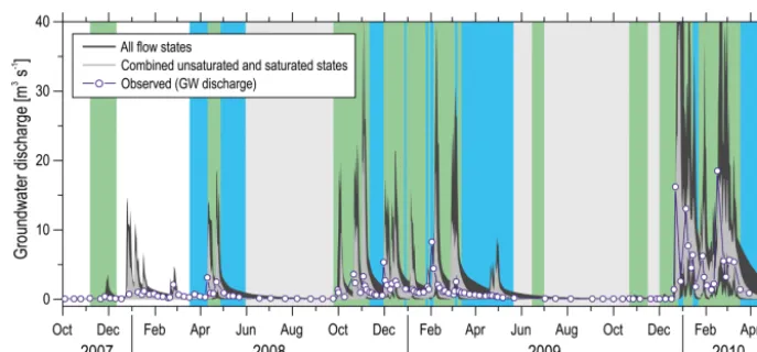
Figure 7.Observed discharge and the simulation uncertainty of the final parameter sample (all KGE≥0.2) of the combined unsaturated and saturated flow states and the all flow states including the disinformative period of river influence. Background colours representing flow states match those in Fig. 2.
stability of NO−3 dynamics within the karst system under ox-idizing conditions (Mudarra et al., 2014), which favours its preservation from surface to the spring.
SO2−4 provided most information on the parameterscSO4,
aSO4, andaSE during the saturated state. This makes sense
as SO2−4 is stored within the saturated zone of the system where groundwater is in touch with gypsum-bearing geolog-ical formations (Triassic clays with evaporites), which are found in contact with deeper aquifer compartments. SO2−4 time series provide more information about the unsaturated zone/epikarst drainage during the saturated flow stage. Such findings mean that the high chemical contrast observed in SO2−4 concentrations of fresh (recently infiltrated) and old (stored) groundwater is useful to assess the relative impor-tance of unsaturated flow and saturated flow during the satu-rated flow stage (Barberá and Andreo, 2015; Mudarra et al., 2011).
The highest number of identifiable parameters is found when all information (discharge, NO−3, and SO2−4 observa-tions) is combined and estimated during the combined un-saturated and un-saturated flow stages (Fig. 6). In addition to the parameters that showed an increase in identifiability at the individual stages (A, VE, KC,VS, KE, aSE, cSO4, and
aSO4), we also see an increased identifiability of the
parame-teraf, most probably due to parameter interactions (Pianosi et al., 2016). OnlyaGWandKEremain with low
identifiabil-ity, which may be due to structural limitations of the model structure (Clark et al., 2008) or due to parameter interactions that are not explicitly considered in our approach. In fact, a lower identifiability ofVE in favour of a high identifiability
of VE was found in a previous study with a similar version
of the model (Hartmann et al., 2015). Compared to that, us-ing all information durus-ing the entire time period, includus-ing the disinformative period, only five of the model parameters show a visible decrease in the distance between the 25th and 75th percentiles of their distribution. Hence, the inclusion of
the disinformative period led to an increase in posterior pa-rameter uncertainty compared to using only the informative time periods represented by the unsaturated and saturated states. This was also shown by Beven and Westerberg (2011) or Beven et al. (2011), when they considered the impact of disinformative discharge events.
The impact of the disinformative time period on the preci-sion of the observations is clearly visible in Fig. 7. Since the model has to compensate for structural errors, i.e. the missing representation of the influence of the river on the discharge of the karst spring, it is forced to allow for a wider range of parameter combinations to account for the simulation errors. Using only the unsaturated and saturated states allows for a much better confinement of model parameters and there-fore a much smaller simulation uncertainty, although show-ing some deviations durshow-ing the periods when the fiver affects the flow system of the spring (blue shaded areas in Fig. 7). Hence, similar to Kauffeldt et al. (2013), our study shows that a proper pre-analysis of the information content of ob-servations for model parameter estimation (Sect. 2.2) allows for excluding disinformative information to reduce model pa-rameter and simulation uncertainty.
5.3 Limits and transferability of the approach
that drains the different aquifer zones (unsaturated zone and saturated zone), and that is affected by the Turón river, can be estimated using EC (Fig. 2), it is rather based on subjec-tive interpretation. However, it can be argued that the previ-ous knowledge based on the accurate interpretation of the El Burgo spring chemographs has permitted a realistic flow de-composition from EC time series as our results show a clear difference in estimated parameter distributions and resulting simulation uncertainty using the unsaturated and saturated flow states and the entire time period including the disinfor-mative data. A more precise distinction between the states is only possible if specific chemical indicators are available to better constrain the differentiation of flow states contribut-ing to the El Burgo sprcontribut-ing discharge, which was not possible within the frame of this study. But even though due to sub-jectivity, the identification of time periods or data sets that contain disinformative contributions to parameter estimation is a useful way to reduce the simulation uncertainty of hydro-logical models. Building on previous research on distive data that focussed on disinformadistive discharge informa-tion, our approach provides a systematic procedure that also includes hydrochemical observations to identify disinforma-tive periods and to improve parameter estimation of models for complex hydrological systems. Another limitation of our research is the low resolution of the discharge and hydro-chemical observations (7–8 days). Although our approach took into account this weakness by the soft rules allowing for remaining uncertainty after the reduction in our 500 000 parameter sets, we believe that a higher resolution of the ob-servations (preferably 1 day) would have resulted in a more pronounced reduction in the initial sample and consequently to a lower remaining uncertainty.
6 Conclusions
In this research, a new approach to estimate the information content of water quality data and the value of identifying most informative periods for model parameter estimation has been proposed. Using soft rules to include discharge, NO−3 and SO2−4 observations into the parameter estimation proce-dure, we were able to reduce an initial sample of 500 000 pa-rameter sets during predefined flow states; one being a known period of disinformative data. Comparing the distributions of the initial and reduced parameter sets, we were able to quan-tify the information contained in our observations to idenquan-tify the parameters of our simulation model.
We found that the information content of the observations varies for the different states that we considered. NO−3 pro-vided most of its information when the unsaturated zone processes dominate the discharge behaviour of the spring. During the time when the saturated zone controls the out-flow behaviour, SO2−4 and discharge observations provide the best information to identify the model parameters. Including the disinformative period, the information content of all data generally decreases, as well as the uncertainty in simulations increases. We finally show that the combination of saturated and unsaturated flow states provides the most precise infor-mation about the model parameters. Due to parameter in-teractions, even model parameters that were not identifiable during the unsaturated or saturated flow state alone became identifiable. As a result, the simulation uncertainty is signif-icantly reduced compared to the simulations obtained by the entire time series of observations that include the disinforma-tive data.
Even though exemplified at a particular karst spring in southern Spain, our approach is easily transferrable to other modelling studies that want to use water quality data for the identification of disinformative periods and for the estimation of model parameters. Our results add to previous findings on the value of removing disinformative data from model pa-rameter estimation to reduce simulation uncertainty. Further-more our results can help building a better communication between experimental hydrologists and modelers (Hartmann, 2016; Seibert and McDonnell, 2002) as hydrochemical data is often used for system characterization. Our study showed that NO−3 and SO2−4 , often used for understanding the un-saturated and un-saturated zone processes, also help to identify the corresponding process parameters in our model. Further research should, therefore, include the evaluation of other hydrochemical variables that can be attributed to particular hydrological processes, and their value to identify the cor-responding processes in process-based simulation models. Also, a further disaggregation of the Kling–Gupta efficiency into its components, correlation, bias, and variability, con-tains high promise for further advancement of our approach.
Appendix A
The parameterVmean,S (mm) and the distribution coefficient
aSE(–) control the variability in soil depths over theNmodel
compartments. Using them, the soil storage capacity VS,i (mm) for every compartmentiis defined by the following:
VS,i=Vmax,S· i
N aSE
. (A1)
Vmax,S (mm) represents the maximum soil storage capacity
and is derived fromVSby the following:
i1/2
R
0
Vmax,Sx N
aSE
dx= N
R
0
Vmax,S NxaSE
dx
2 ;VS=Vmax,S
i
1/2 N
aSE
m
Vmax,S=VS·2 a
SE
aSE+1
,
(A2) where the compartment at which the volumes on the left equal the volumes on the right is found ati1/2. The same
dis-tribution coefficientaSEis used to derive the epikarst storage
distribution by the mean epikarst depthVE(mm) (derivation
ofVmax,Elikewise toVmax,Sin Eq. 4)
VE,i=Vmax,E· i
N aSE
. (A3)
Actual evapotranspiration from each soil compartmentEact,i is calculated by
Eact,i(t )=Epot(t ) (A4)
·min
VSoil,i(t )+P (t )+QSurface,i(t ) , VS,i
VS,i
.
Potential evapotranspiration Epot (mm) is found by the
Thornthwaite equation (Thornthwaite, 1948) and Qsurface,i (mm) is the surface inflow that originates from compartment
i−1 (see Eq. 11).VSoil,i(mm) is the volume of water stored in the soil at time stept. Recharge from the soil to the epikarst
REpi,i(mm) is found by water balance
REpi,i(t )=Qinf(t )+max (A5)
VSoil,i(t )+P (t )+QSurface,i(t )−Eact,i(t )−VS,i,0, withQinf(t )being the river infiltration (Eq. 5). The epikarst
storage coefficient KE,i (d) controls the outflow from the epikarst
QEpi,i(t )= min
VEpi,i(t )+REpi,i(t ) , VE,i
KE,i
·1t, (A6)
KE,i=Kmax,E·
N−i+1 N
aSE
. (A7)
Here,VEpi,i (mm) is the water stored in the epikarst at time stept.Kmax,E is found by the mean epikarst storage
coef-ficientVEand by applying the same distribution coefficient
aSE
N·KE=
N
R
0
Kmax,E x
N aSE
dx m
Kmax,E=KE·(aSE+1) .
(A8)
Surface flow to the next model compartmentQSurf,i+1(mm)
initiates when soil and epikarst storage capacities are ex-ceeded:
QSurf,i+1(t )=max
VEpi,i(t )+REpi,i(t )−VE,i,0
. (A9)
The vertical percolation from the epikarst is split into dif-fuse (Rdiff,i, mm) and concentrated groundwater recharge (Rconc,i, mm) again by a variable separation factorfC,i (–) and a distribution coefficientaf (–)
Rconc,i(t )=fC,i·QEpi,i(t ) , (A10)
Rdiff,i(t )= 1−fC,i
·QEpi,i(t ) , (A11)
fC,i=
i
N af
. (A12)
The diffuse recharge reaches the groundwater compartments (i=1. . .N−1) directly below, while concentrated recharge is routed laterally to the conduit system (compartmenti=N). Similar to epikarst storage coefficients, variable groundwater storage coefficientsKGW,i (d) are calculated. The, ground-water contributions of the matrix system QGW,i (mm) in therefore found by the following:
QGW,i(t )=
VGW,i(t )+Rdiff,i(t )
KGW,i
;i=1. . .N−1, (A13)
with
KGW,i=KC· i
N −aGW
. (A14)
The conduit system discharges from compartmentN
QGW,i(t )=
VGW,N(t )+ N
P
i=1
Rconc,i(t )
KC
;i=N, (A15) where the conduit storage coefficient is given by KC (d).
The discharge of the main springQmain(L s−1) is comprised
of the sum of the matrix and the conduit system discharge rescaled to L s−1units the recharge areaA(km2)
Qmain(t )=
A
N ·
N
X
i=1
Solute transport within the VarKarst model follows the as-sumption of complete mixing for every model compartment. Hence, enrichment only takes place due to evaporation and by geogenic dissolution (only SO2−4 ), for which varying equilibrium concentrations are defined according to
cSO4,i=cmax,SO4·
N−i+1 N
aSO4
, (A17)
whereaSO4 is a variability constant andcmax,SO4 is derived
fromcSO4 (mg L
Competing interests. The authors declare that they have no conflict of interest.
Acknowledgements. This work is a contribution to the projects P06-RNM 2161 of Junta de Andalucía; and CGL2008-06158 BTE, CGL2012-32590, CGL2015-65858-R of DGICYT; and to the Research Group RNM-308 of the Junta de Andalucía. The article processing charge was funded by the German Research Foundation (DFG) and the University of Freiburg in the funding programme Open Access Publishing.
Edited by: Matthias Bernhardt
Reviewed by: Naomi Mazzilli and Arnauld Malard
References
Aquilina, L., Ladouche, B., Dörfliger, N., and Doerfliger, N.: Water storage and transfer in the epikarst of karstic systems during high flow periods, J. Hydrol., 327, 472–485, 2006.
Bakalowicz, M.: Karst groundwater: a challenge for new resources, Hydrogeol. J., 13, 148–160, https://doi.org/10.1007/s10040-004-0402-9, 2005.
Barberá, J. A.: Hydrogeological research in the carbonate aquifers of eastern Serranía de Ronda (Málaga) in Spanish and English, PhD thesis at the Centre of Hydrogeology of the University of Málaga CEHIUMA (Spain), 2014.
Barberá, J. A. and Andreo, B.: Hydrogeological characterization of two karst springs in southern Spain by hydrochemical data and intrinsic natural fluorescence, in: IAH Selected Papers – Groundwater Quality Sustainability, edited by: Maloszewski, P., Witczak, S., and Malina, G., Vol. 17, 281–295, ISBN:978-0-415-69841-2, 2012.
Barberá, J. A. and Andreo, B.: Hydrogeological processes in a fluviokarstic area inferred from the analysis of nat-ural hydrogeochemical tracers. The case study of eastern Serranía de Ronda (S Spain), J. Hydrol., 523, 500–514, https://doi.org/10.1016/j.jhydrol.2015.01.080, 2015.
Beven, K. and Westerberg, I.: On red herrings and real herrings: Disinformation and information in hydrological inference, Hy-drol. Process., 25, 1676–1680, https://doi.org/10.1002/hyp.7963, 2011.
Beven, K., Smith, P. J., and Wood, A.: On the colour and spin of epistemic error (and what we might do about it), Hydrol. Earth Syst. Sci., 15, 3123–3133, https://doi.org/10.5194/hess-15-3123-2011, 2011.
Beven, K. J.: A manifesto for the equifinality thesis, J. Hydrol., 320, 18–36, 2006.
Brenner, S., Coxon, G., Howden, N. J. K., Freer, J., and Hartmann, A.: A percentile approach to evaluate simulated groundwater levels and frequencies in a Chalk catchment in Southwest England, Nat. Hazards Earth Syst. Sci. Discuss., https://doi.org/10.5194/nhess-2016-386, in review, 2016. Charlier, J.-B., Bertrand, C., and Mudry, J.: Conceptual
hydro-geological model of flow and transport of dissolved organic carbon in a small Jura karst system, J. Hydrol., 460–461, https://doi.org/10.1016/j.jhydrol.2012.06.043, 2012.
Choi, H. T. and Beven, K.: Multi-period and multi-criteria model conditioning to reduce prediction uncertainty in an application of TOPMODEL within the GLUE framework, J. Hydrol., 332, 316–336, https://doi.org/10.1016/j.jhydrol.2006.07.012, 2007. Clark, M. P., Slater, A. G., Rupp, D. E., Woods, R. A., Vrugt, J. A.,
Gupta, H. V, Wagener, T., and Hay, L. E.: Framework for Under-standing Structural Errors (FUSE): A modular framework to di-agnose differences between hydrological models, Water Resour. Res., 44, W00B02, https://doi.org/10.1029/2007WR006735, 2008.
Cruz-Sanjulián, J. J.: Estudio geológico del sector Cañete la Real-Teba-Osuna (Cordillera Bética, región occidental), PhD thesis, Universidad de Granada, 374 pp., 1974.
Fernández, R.: Investigaciones hidrogeológicas al Norte de Ronda (Málaga), Granada, Simposio del Agua en Andalucía 2, 643– 658, 1980.
Ford, D. C. and Williams, P. W.: Karst Hydrogeology and Geomor-phology, John Wiley & Sons, Wiley, Chichester, United King-dom, 567 pp., ISBN:978-0-470-84996-5, 2007.
Ghasemizadeh, R., Hellweger, F., Butscher, C., Padilla, I., Vesper, D., Field, M., and Alshawabkeh, A.: Review: Groundwater flow and transport modeling of karst aquifers, with particular refer-ence to the North Coast Limestone aquifer system of Puerto Rico, Hydrogeol. J., 20, 1441–1461, https://doi.org/10.1007/s10040-012-0897-4, 2012.
Goldscheider, N. and Drew, D.: Methods in Karst Hydrogeology, edited by: I. A. of Hydrogeologists, Taylor & Francis Group, Lei-den, NL, ISBN:978-0-415-42873-6, 2007.
Gupta, H. V., Kling, H., Yilmaz, K. K., and Martinez, G. F.: Decom-position of the mean squared error and NSE performance criteria: Implications for improving hydrological modelling, J. Hydrol., 377, 80–91, https://doi.org/10.1016/j.jhydrol.2009.08.003, 2009. Hartmann, A.: Putting the cat in the box: why our models should consider subsurface heterogeneity at all scales, WIREs Water, https://doi.org/10.1002/wat2.1146, 2016.
Hartmann, A. and Baker, A.: Modelling karst vadose zone hydrol-ogy and its relevance for paleoclimate reconstruction, Earth-Sci. Rev., 1–54, https://doi.org/10.1016/j.earscirev.2017.08.001, 2017.
Hartmann, A., Lange, J., Weiler, M., Arbel, Y., and Greenbaum, N.: A new approach to model the spatial and temporal variability of recharge to karst aquifers, Hydrol. Earth Syst. Sci., 16, 2219– 2231, https://doi.org/10.5194/hess-16-2219-2012, 2012. Hartmann, A., Weiler, M., Wagener, T., Lange, J., Kralik, M.,
Humer, F., Mizyed, N., Rimmer, A., Barberá, J. A., Andreo, B., Butscher, C., and Huggenberger, P.: Process-based karst mod-elling to relate hydrodynamic and hydrochemical characteristics to system properties, Hydrol. Earth Syst. Sci., 17, 3305–3321, https://doi.org/10.5194/hess-17-3305-2013, 2013a.
Hartmann, A., Barberá, J. A., Lange, J., Andreo, B., Weiler, M., An-tonio, J., Lange, J., Andreo, B., Weiler, M., Barberá, J. A., Lange, J., Andreo, B., and Weiler, M.: Progress in the hydrologic simula-tion of time variant recharge areas of karst systems – Exemplified at a karst spring in Southern Spain, Adv. Water Res., 54, 149– 160, https://doi.org/10.1016/j.advwatres.2013.01.010, 2013b. Hartmann, A., Goldscheider, N., Wagener, T., Lange, J., and Weiler,
Hartmann, A., Mudarra, M., Andreo, B., Marín, A., Wagener, T., and Lange, J.: Modeling spatiotemporal impacts of hy-droclimatic extremes on groundwater recharge at a Mediter-ranean karst aquifer, Water Resour. Res., 50, 6507–6521, https://doi.org/10.1002/2014WR015685, 2014b.
Hartmann, A., Gleeson, T., Rosolem, R., Pianosi, F., Wada, Y., and Wagener, T.: A large-scale simulation model to assess karstic groundwater recharge over Europe and the Mediterranean, Geosci. Model Dev., 8, 1729–1746, https://doi.org/10.5194/gmd-8-1729-2015, 2015.
Hartmann, A., Kobler, J., Kralik, M., Dirnböck, T., Humer, F., and Weiler, M.: Model-aided quantification of dissolved carbon and nitrogen release after windthrow disturbance in an Austrian karst system, Biogeosciences, 13, 159–174, https://doi.org/10.5194/bg-13-159-2016, 2016.
Hartmann, A., Gleeson, T., Wada, Y., Wagener, T., Kingdom, U., Sciences, O., and Kingdom, U.: Enhanced groundwater recharge rates and altered recharge sensitivity to climate variabil-ity through subsurface heterogenevariabil-ity, P. Natl. Acad. Sci. USA, 19, EGU2017-12796, https://doi.org/10.1073/pnas.1614941114, 2017.
Hunkeler, D. and Mudry, J.: Hydrochemical tracers, Methods in karst hydrogeology, edited by: Goldscheider, N. and Drew, D., 93–121, Taylor and Francis/Balkema, London, UK, 2007. Jakeman, A. J. and Hornberger, G. M.: How much complexity is
warranted in a rainfall-runoff model?, Water Resour. Res., 29, 2637–2649, 1993.
Kauffeldt, A., Halldin, S., Rodhe, A., Xu, C.-Y., and West-erberg, I. K.: Disinformative data in large-scale hydrolog-ical modelling, Hydrol. Earth Syst. Sci., 17, 2845–2857, https://doi.org/10.5194/hess-17-2845-2013, 2013.
Kovacs, A. and Sauter, M.: Modelling karst hydrodynamics, Meth-ods in karst hydrogeology, edited by: Goldscheider, N. and Drew, D., 65–91, Taylor and Francis/Balkema, London, UK, 2007. Kuczera, G. and Mroczkowski, M.: Assessment of hydrologic
pa-rameter uncertainty and the worth of multiresponse data, Water Resour. Res., 34, 1481–1489, 1998.
Labat, D., Ababou, R., and Mangin, A.: Rainfall-runoff relations for karstic springs. Part I: convolution and spectral analyses, J. Hydrol., 238, 123–148, 2000.
Martín-Algarra, A.: Evolución geológica Alpina del contacto entre las Zonas Internas y las Zonas Externas de la Cordillera Bética (Sector Occidental), Universidad de Granada, 1987.
Mazzilli, N., Jourde, H., Jacob, T., Guinot, V., Moigne, N., Boucher, M., Chalikakis, K., Guyard, H., and Legtchenko, A.: On the in-clusion of ground-based gravity measurements to the calibration process of a global rainfall-discharge reservoir model: case of the Durzon karst system (Larzac, southern France), Environ. Earth Sci., 68, 1631–1646, https://doi.org/10.1007/s12665-012-1856-z, 2012.
Mudarra, M., Andreo, B., and Mudry, J.: Monitoring groundwater in the discharge area of a complex karst aquifer to assess the role of the saturated and unsaturated zones, Environ. Earth Sci., 65, 2321–2336, https://doi.org/10.1007/s12665-011-1032-x, 2011.
Mudarra, M., Andreo, B., Marína, I., Vadillo, I., and Barberá, J. A.: Combined use of natural and artificial tracers to determine the hydrogeological functioning of a karst aquifer: the Villanueva del Rosario system (Andalusia, southern Spain), Hydrogeol. J., 22, 1027–1039, https://doi.org/10.1007/s10040-014-1117-1, 2014. Oehlmann, S., Geyer, T., Licha, T., and Sauter, M.: Reducing the
ambiguity of karst aquifer models by pattern matching of flow and transport on catchment scale, Hydrol. Earth Syst. Sci., 19, 893–912, https://doi.org/10.5194/hess-19-893-2015, 2015. Perrin, C., Michel, C., and Andréassian, V.: Improvement of a
parsi-monious model for streamflow simulation, J. Hydrol., 279, 275– 289, 2003.
Pianosi, F., Beven, K., Freer, J., Hall, J. W., Rougier, J., Stephenson, D. B., and Wagener, T.: Sensitivity analy-sis of environmental models: A systematic review with practical workflow, Environ. Model. Softw., 79, 214–232, https://doi.org/10.1016/j.envsoft.2016.02.008, 2016.
Reusser, D. E. and Zehe, E.: Inferring model structural deficits by analyzing temporal dynamics of model perfor-mance and parameter sensitivity, Water Resour. Res., 47, https://doi.org/10.1029/2010wr009946, 2011.
Rimmer, A. and Hartmann, A.: Optimal hydrograph separation filter to evaluate transport routines of hydrological models, J. Hydrol., 514, 249–257, https://doi.org/10.1016/j.jhydrol.2014.04.033, 2014.
Sauter, M., Kovács, A., Geyer, T., and Teutsch, G.: Modellierung der Hydraulik von Karstgrundwasserleitern – Eine Übersicht, Grundwasser, 3, 143–156, 2006.
Seibert, J. and McDonnell, J. J.: On the dialog between experimen-talist and modeler in catchment hydrology: Use of soft data for multicriteria model calibration, Water Resour. Res., 38, 1241, https://doi.org/10.1029/2001WR000978, 2002.
Son, K. and Sivapalan, M.: Improving model structure and re-ducing parameter uncertainty in conceptual water balance mod-els through the use of auxiliary data, Water Resour. Res., 43, W01415, https://doi.org/10.1029/2006wr005032, 2007. Thornthwaite, C. W.: An Approach toward a
Ratio-nal Classification of Climate, Geogr. Rev., 38, 55–94, https://doi.org/10.2307/210739, 1948.
Wagener, T., McIntyre, N., Lees, M. J., Wheater, H. S., and Gupta, H. V: Towards reduced uncertainty in conceptual rainfall-runoff modelling: dynamic identifiability analysis, Hydrol. Process., 17, 455–476, https://doi.org/10.1002/hyp.1135, 2003.
Wheater, H. S., Bishop, K. H., and Beck, M. B.: The iden-tification of conceptual hydrological models for sur-face water acidification, Hydrol. Process., 1, 89–109, https://doi.org/10.1002/hyp.3360010109, 1986.
White, W. B. and White, E. L.: Ground water flux distribution be-tween matrix, fractures, and conduits?: constraints on modeling, Speleogenesis and Evolution of Karst Aquifers, 3, 1–6, 2003. Ye, W., Bates, B. C., Viney, N. R., Sivapalan, M., and Jakeman,