Development and evaluation of a global dynamical wetlands extent scheme

www.hydrol-earth-syst-sci.net/16/2915/2012/ doi:10.5194/hess-16-2915-2012

© Author(s) 2012. CC Attribution 3.0 License.

Earth System

Sciences

Development and evaluation of a global dynamical wetlands

extent scheme

T. Stacke and S. Hagemann

Max-Planck-Institut f¨ur Meteorologie, Bundesstraße 53, 20146 Hamburg, Germany Correspondence to: T. Stacke ([email protected])

Received: 13 December 2011 – Published in Hydrol. Earth Syst. Sci. Discuss.: 10 January 2012 Revised: 30 July 2012 – Accepted: 30 July 2012 – Published: 23 August 2012

Abstract. In this study we present the development of the dynamical wetland extent scheme (DWES) and evaluate its skill to represent the global wetland distribution. The DWES is a simple, global scale hydrological scheme that solves the water balance of wetlands and estimates their extent dynam-ically. The extent depends on the balance of water flows in the wetlands and the slope distribution within the grid cells. In contrast to most models, the DWES is not directly cali-brated against wetland extent observations. Instead, wetland affected river discharge data are used to optimise global pa-rameters of the model. The DWES is not a complete hydro-logical model by itself but implemented into the Max Planck Institute – Hydrology Model (MPI-HM). However, it can be transferred into other models as well.

For present climate, the model evaluation reveals a good agreement for the spatial distribution of simulated wetlands compared to different observations on the global scale. The best results are achieved for the Northern Hemisphere where not only the wetland distribution pattern but also their ex-tent is simulated reasonably well by the DWES. However, the wetland fraction in the tropical parts of South America and Central Africa is strongly overestimated. The simulated extent dynamics correlate well with monthly inundation vari-ations obtained from satellites for most locvari-ations. Also, the simulated river discharge is affected by wetlands resulting in a delay and mitigation of peak flows. Compared to sim-ulations without wetlands, we find locally increased evapo-ration and decreased river flow into the oceans due to the implemented wetland processes.

In summary, the evaluation demonstrates the DWES’ abil-ity to simulate the distribution of wetlands and their seasonal variations for most regions. Thus, the DWES can provide hy-drological boundary conditions for wetland related studies.

In future applications, the DWES may be implemented into an Earth system model to study feedbacks between wetlands and climate.

1 Introduction

In recent studies wetlands are suspected to play an important role during periods of climate change (e.g. Ringeval et al., 2011; Gedney et al., 2004; Levin et al., 2000). However, the representation of the wetland’s spatial extent and its tempo-ral variations is still a weak point in today’s Earth System Models (ESMs) and needs to be improved by a better sim-ulation of their hydrological cycle (O’Connor et al., 2010; Ringeval et al., 2010). Besides the wetland extent, the water level is an important factor for the wetland’s biogeochemistry which results in carbon sequestration or decomposition (e.g. O’Connor et al., 2010, and references therein). In the satu-rated soil zone, below the water table, anoxic conditions pre-vail which are favourable for methane producing microbes. Depending on factors like temperature, available substrate and pH, organic material is decomposed and methane is pro-duced. While methane diffuses upwards, it can be oxidised to CO2within the unsaturated oxic soil zone above the

However, even without consideration of the carbon cycle, the wetland hydrology in itself is an important key factor in the climate system. Wetlands are often related to regions with open surface water and saturated soil. Such regions have to be considered in ESMs because of their potential feedbacks to the atmosphere (Coe and Bonan, 1997). The effect of open water surfaces on the energy and water balance was investi-gated by several modelling studies, e.g. Bonan (1995) and Mishra et al. (2010), who reported a significant impact of wetlands on the local climate. Generally, they found a cool-ing of the surface temperature in wetland dominated regions due to increased evapotranspiration (ET), as well as an in-crease in the latent heat flux and a dein-crease in the sensible heat flux. Eventually, this could result in increased precipi-tation rates as shown by Coe and Bonan (1997) and Krin-ner et al. (2012). Furthermore, wetlands interact in several ways with the hydrological cycle of their surrounding area. They are commonly expected to regulate river flow, mitigate flood events and recharge groundwater. These observations are consistent with a modelling study by Mishra et al. (2010) who found decreased surface runoff in wetland dominated regions. However, a number of studies exists that describe the opposite behaviour (Bullock and Acreman, 2003). All of these processes are of great interest for impact studies that in-vestigate how climate change might effect the water storage capacities in a region or the characteristics of river flooding. In our study we focus on modelling the hydrological cy-cle in wetlands and their extent dynamics, which we see as a prerequisite for the computation of the wetland carbon cycle. This issue already motivated a large number of modelling studies. Generally, most models follow one of two main ap-proaches for the hydrological representation of wetlands.

One approach is concerned with the redistribution of soil moisture in the model grid cell. A widely used exam-ple is TOPMODEL (Beven and Kirkby, 1979). In this ap-proach a topographical index is computed that depends on the drainage of a given area routed through a point and its slope. This index is then applied to determine the position of the local water table at that point relative to the mean wa-ter table of the whole grid cell. The grid cell fraction where the sub-grid soil moisture exceeds the soil moisture storage capacity of the grid cell is then regarded as a wetland. The TOPMODEL approach is used and improved in several stud-ies (e.g. Barling et al., 1994; Gedney et al., 2004; Bohn et al., 2007; Kleinen et al., 2012) and able to compute changes in wetland extent as well. While this approach is an elegant so-lution, we see in it one major problem. As the wetland frac-tion depends on the redistribufrac-tion of the mean grid cell soil moisture, it follows that there is an upper boundary for the maximum water depth and wetland fraction. For the extreme case of a grid cell with zero slope no wetland can emerge because the mean soil moisture can obviously not exceed the maximum soil moisture capacity. However, observations in-dicate that flat regions appear to be more suitable for wetland formation.

The second approach is the explicit modelling of surface water. In this case depressions in the topography are identi-fied and filled with water that results from a positive water balance. On the one hand, this can be done on a continen-tal scale (e.g. Coe, 1997, 1998, 2000) but then the quality of the wetland representation is strongly limited by resolu-tion of the model. Alternatively, regional models allow for a higher resolution but then depend strongly on detailed soil property information (e.g. Bowling and Lettenmaier, 2010; Yu et al., 2006) or are calibrated for specific catchments (e.g. Bohn et al., 2007). Decharme et al. (2008, 2011) developed a global inundation model, but its focus is concentrated on the representation of floodplains.

In contrast to these sophisticated approaches, we wanted to develop a more simple hydrological scheme that represents the global distribution and extent variability of very different types of wetlands. The scheme is designed for the applica-tion in complex ESMs on global scale with medium to coarse resolutions (50 km or coarser), because we think that the rep-resentation of surface water dynamics is – albeit important – not strongly developed in such models. While an explicit representation of wetland dynamics is necessary for the cal-culation of CH4emissions, we also expect an improved

simu-lation of the hydrological cycle due to our scheme. From this objective several limitations arise. Of course, we strive for a realistic representation of wetland extent but nevertheless our approach needs to be simple. It should be easily imple-mentable into different ESMs and should only require bound-ary data that is readily available on global scale. By these means, we want to minimise the necessity to recalibrate our model parameters for different applications or setups of the ESM in order to allow for future projections and hindcast ex-periments as well as for present day simulations. Therefore, we restrict our scheme to the use of the general water balance terms, which are considered in all ESMs, and topographical data, which is globally available. One example for an already existing wetland model of similar complexity is the study of Krinner (2003). The author relates wetland extent dynami-cally to the total quantity of water in wetlands and the mean topographic index of the grid cell. However, they prescribe their wetland dynamics with an upper boundary based on observation and do not consider any horizontal surface water routing between grid cells. In our study we want to overcome these limitations.

2 Model development

The DWES is not a stand alone model by itself but needs to be implemented into a large scale model. Instead of starting the model development directly within the framework of an ESM, the Max Planck Institute – Hydrology Model (MPI-HM) was chosen as a test environment for the development of the DWES. The MPI-HM computes the global water cycle only and thus it is possible to investigate the direct effects of the DWES before indirect effects due to interactions with other ESM components occur.

2.1 The MPI-HM

The MPI-HM is a global hydrological model which solves the land surface water balance at a horizontal resolution of 0.5◦_{with a time step of 1 day. It is restricted to the} computa-tion of water fluxes and does not consider any energy balance calculations. The MPI-HM consists of two formerly sepa-rated sub-components, the Simplified Land surface Scheme (SL-Scheme) (Hagemann and D¨umenil Gates, 2003) and the Hydrological Discharge Model (HD-Model) (Hagemann and D¨umenil, 1998, 1999; Hagemann and D¨umenil Gates, 2001). The SL-Scheme includes a simple snow scheme based on the degree day approach (e.g. Rango and Martinec, 1995) and uses a soil bucket scheme for the computation of the ver-tical water balance. Most of its water flux calculations are functions of the relative saturation of the soil storage. The main outputs of the SL-Scheme are daily fields of runoff and drainage. These are given to the HD-Model, which is a state of the art river routing model. It computes the retention time of water in overflow, baseflow and riverflow reservoirs using a linear reservoir cascade (Singh, 1988). Horizontal outflow from a storage is given to the river flow reservoir of the down-stream grid cell. The river flow net is computed based on ele-vation data and manually adjusted for major catchments. As wetlands are subject to vertical as well as horizontal water fluxes simultaneously, both water balances have to be solved during every model time step. Thus, the SL-Scheme and HD-Model were coupled to form the MPI-HM.

The MPI-HM requires daily temperature and precipitation data as climate forcing. Both data fields were taken from the WATCH Forcing Data (WFD) (Weedon et al., 2011) which is a quasi-observational dataset. Optionally, it is possible to use prescribed forcing for potential evapotranspiration (PET) instead of relying on the native PET calculation in the MPI-HM, which is based on the Thornthwaite formula (Thornth-waite and Mather, 1955). In order to derive PET forcing that is consistent with the WFD, we adopted the Weedon et al. (2011) method for PET calculation and applied the Penman-Monteith reference ET as proxy for PET. Following their study and the FAO recommendations (Allen et al., 1998) we used globally constant parameters of short grass for the crop height and aerodynamic resistance.

In this study all simulations were conducted for the period 1958–1999. The first five years are used to spin-up different MPI-HM storages and are excluded from the optimisation and the analysis of the results.

2.2 Wetland dynamics

In our approach, wetlands are defined as the occurrence of surface water that covers a certain area fraction in a model grid cell. Following our simplicity criteria, we decided not to differentiate the treatment of different wetland types and lakes but to use a general approach instead. For this approach we make two preconditions: first, that wetland formation re-quires excess water on the land surface and second, that wet-lands form preferentially on the flat parts of a grid cell.

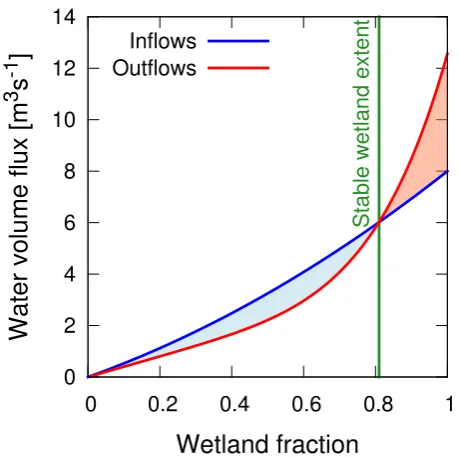
As starting point for the parametrization of wetland dy-namics we assume that the water balance of a wetland de-pends directly on its surface extent. For example, a wetland with a small surface extent would loose less water volume due to open water evaporation than a larger wetland. How-ever, a small wetland would also gain less water volume from horizontal inflow than a larger wetland, because a small wet-land is easily bypassed by rivers in this region. Analysing the water balance fluxes separately, we see that the volume of vertical water fluxes (e.g. precipitation, evaporation and drainage) depend linearly on the wetland extent. However, horizontal fluxes (e.g. river inflow from upstream grid cells or outflow from the wetland) have a more complex, non-linear relation with the wetland extent as explained in the detailed discussion of the wetland water balance in Sect. 2.3. Thus, the overall wetland inflowI (Eq. 1) and outflowO (Eq. 2) at a given time stepiare sums of water flows which depend on wetland extent in a linear as well as a non-linear manner. They are indicated with the subscriptsl for linear flows and

nfor non-linear flows, respectively. Ii =

X Ii,l+

X

Ii,n (1)

Oi = X

Oi,l+ X

Oi,n (2)

0

2

4

6

8

10

12

14

0

0.2

0.4

0.6

0.8

1

Wa

ter volu

me flu

x [m

3

s

-1

]

Wetland fraction

Stable wetland extent

Inflows

Outflows

Fig. 1. Conceptual sketch of wetland water inflows (blue curve) and

outflows (red curve) in dependence on the wetland’s surface area. The stable wetland extent (green line) is found on the intersection of both curves and depend on climatic forcing during the respective model time step and the topography of the grid cell. The blue shaded area indicates excess water if the inflow exceeds the outflow and vice versa for the red shaded area.

wetland extent response times in respect to changes in the climatic conditions. Thus, wetland formation is promoted on low slopes and suppressed on steeper regions. The ef-fect is further enhanced because steeper slopes also increase the amount of horizontal wetland outflow (see Sect. 2.3). In order to consider slope information in our approach, highly resolved topographical information is required. Such infor-mation is available in the GTOPO30 dataset (Gesch et al., 1999) which provides elevations for the global land surface at 30 arc sec horizontal resolution. Based on these data, slope information were derived resulting in 3600 slope values for every 0.5° sized grid cell of the MPI-HM. As this amount of information would increase the computational requirements of the MPI-HM significantly, we had to represent the slope information in a reduced way. First, the sub-grid slope values for every grid cell were sorted. Thus, the slope is directly re-lated to the grid cell fraction as shown in Fig. 2. Furthermore, the fraction–slope relation was approximated using Eq. (3). This equation is a modified version of the formula that was successfully used by Hagemann and D¨umenil Gates (2003) to account for grid heterogeneity. The maximum sub-grid slopes(f )for the grid cell fractionf can be described as

s(f )=MAXh1−(1−f )1b

·srange+smin,0

i

, with (3) srange=smax−smin

0.00

0.02

0.04

0.06

0.08

0.10

0.12

0.14

0.16

0.18

0

0.2

0.4

0.6

0.8

1

Slo

pe [m/m

]

Grid cell fraction [ ]

Slope data

Slope function

Fig. 2. Maximum sub-grid slopes that occurs for a given grid cell

fraction. The grey area displays discrete slope data derived from the GTOPO30 dataset for an example MPI-HM grid cell. The red line displays an analytical approximation of these data based on Eq. (3).

whereb is a shape parameter accounting for the curvature of the curve and srange is the difference between the

max-imum slopesmaxand minimum slope smin of the grid cell.

Whilesmax andsmincan be derived directly from the data, bneeds to be derived by least-squares fitting. For the major-ity of grid cells, this function can be fitted very well to the sub-grid slope distribution with an asymptotic standard error below 1 %.

In the DWES the stable wetland extent is not computed analytically. Instead, only the change in wetland extent is es-timated using an iterative procedure based on the residuum 1V of the water balance calculation (1V =P

1Sof Eq. 6). In Eq. (4) we relate the relative change of the wetland wa-ter volume V to the relative change in wetland extent fw.

Thus, we ensure that the amount of wetland extent change is adjusted to the mismatch between the actual wetland ex-tent and the stable exex-tent where the water balance residuum would converge against zero. The change in wetland extent 1fwis then computed as

1fw = 1V

V ×τ× 1 fw

, with (4)

τ = 1

1+s(fw)×κ

(5) whereτ describes the resistance against a change in wetland extent due to the effect of the maximum slopes(fw)covered

model grid cells,fw is initialised with a minimum grid cell

fraction that is the larger value of either 1×10−10_{or the grid}

cell fraction with zero slope.

An additionally constraint for1fw is given by the

wet-land water level h. The level h is the height of the water column above the soil surface. Its average value is given as h=V / fw×AgcwithAgcas grid cell area. In case of

wet-land growthfwis only allowed to increase by a fraction that

does not decreasehand vice versa for a shrinking wetland. This constrain promotes a steady change in wetland extent and prevents strong oscillations around the stable extent. 2.3 Wetland water balance

The DWES does not explicitly distinguish between differ-ent kinds of wetlands. However, it is useful for the compre-hensibility of our approach to focus the explanation of water balance calculation on the two extremes in the range of wet-land types. Being restricted to hydrological indices, wetwet-land types differ only in the relation of their water fluxes. A dom-ination of vertical water fluxes leads to the formation of sat-urated wetlands. These are usually located in regions where precipitation exceeds evaporation. In contrast, a domination of horizontal water fluxes results in floodplains. They form close to rivers due to inundation. Most wetland models focus on the simulation of either saturated wetlands (e.g. Krinner, 2003; Gedney et al., 2004; Kleinen et al., 2012) or flood-plains (Decharme et al., 2008, 2011). Thus, a key feature of the DWES is that we couple sub-models for the calculation of both, vertical and horizontal, water fluxes to allow for the simultaneous computation of both processes as well as con-sider wetlands which are intermediate between the water flux regimes.

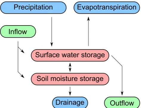
The general wetland water balance is given by Eq. (6) and displayed in Fig. 3. The change in the soil moisture and sur-face water storagesP

1Sfor a given time periodtis given by the balance of inflowing and outflowing wetland water fluxes as

X

1S=(P−ET−D+I−O)×1t (6)

whereP is precipitation, ET is evapotranspiration,Dis sub-surface drainage, andIandOare the horizontal inflows and outflows of water, respectively. As all fluxes are computed as volumes,P

1S equals the water balance residuum1V that is required in Eq. (4) for the computation of wetland dynamics.

Saturated wetlands are dominated by the first three terms of Eq. (6). Their computation is strongly based on the rou-tines of the former SL-Scheme part of the MPI-HM. First, precipitation forcing is separated into rainfall and snowfall depending on surface air temperature. Only liquid precip-itation is then allowed to enter the wetland fraction of the grid cell. Depending on its relative soil moisture content, ET and drainage are computed such that they converge against PET and the maximum drainage value when the soil moisture

Fig. 3. Wetland water balance as simulated by the DWES. The green

boxes indicate horizontal water flows, the blue ones indicate vertical water flows, and the red ones indicate water storages. Please note that horizontal inflow can fill the soil moisture storage as well as the surface water storage of the wetlands. However, horizontal outflow is only generated during periods when surface water exists in the respective wetland.

storage converges against the field capacity. Only then, sur-face water is allowed to build up in the grid cell. While PET is computed using the Penman-Monteith equation (Allen et al., 1998; Weedon et al., 2011), the maximum drainage value had to be estimated. Our estimate is based on the average residuum R of the precipitation – PET difference for all grid cells which are known to contain wetlands in today’s observations. Assuming that these wetlands are hydrologi-cally stable under the current climatic condition, the average drainage must not exceedR because otherwise the wetland would dessicate. Horizontal flows are neglected in this case. Thus, the maximum drainage value is set toR. It corresponds to about 10 % of the maximum drainage value for the non-wetland grid cells. As the MPI-HM lacks an energy balance, it is difficult to account for the freezing of wetlands. In the MPI-HM, only precipitation is affected by low temperatures. Below 3.3◦C, some part of the precipitation is treated as snow. The fraction is gradually increasing and reaches 100 % below−1.1◦_{C. While rainfall is added to the wetland} wa-ter balance at once, the input of snowfall is delayed. Snow is stored on the wetland surface as if the wetland would be frozen and it is only allowed to enter the wetland water bal-ance as melt water. Snow melt is calculated based on the de-gree day approach (e.g. Rango and Martinec, 1995) similar to the original SL-Scheme routines. All other processes are treated similar during frost and no frost periods.

In contrast to saturated wetlands, floodplains are domi-nated by horizontal water flows. These flows are computed by the HD-Model part of the MPI-HM. Every grid cell re-ceives a certain inflowIgcthat is generated by its upstream

grid cells. Igc has to be separated into the inflow I that

reaches the wetland and the inflowIrthat remains in the river.

To our knowledge, no observations are available about the distribution of river flow into all surface water bodies of a grid cell sized area at a resolution of 0.5°×0.5°. However, even if such data were available for some regions, we doubt that it could be used to derive a separation parametrization for the whole land surface. Thus, we tried a simple concept to find a useful and globally applicable parametrization for this separation. Our basic reasoning is that the ratio of horizon-tal inflow into the wetland depends on the amount of overall grid cell inflowIgcand the wetland covered grid cell fraction fw. While a very small wetland will get almost no inflow

and a grid cell size wetland will get it all, the associated rela-tion in between these two extremes is not clear. Two simple approaches were tested for this relation: an exponential func-tion (Eq. 7) and a tanh funcfunc-tion (Eq. 8).

I=Igc×fwz (7)

I=I_gc×min [(tanh(4×π×(f_w−0.5))+1)×0.5,1.0] (8) These functions can be interpreted as follows. Exponents z <1 in Eq. (7) results in a large ratio of inflow already for small wetlands meaning that wetlands are usually close to the rivers and store a considerable amount of water even while being small. For exponentsz >1, the inflow ratio increase is shifted to large wetlands indicating that water flow would be confined to river channels and bypass the wetlands. The tanh function (Eq. 8) would indicate a tipping point meaning that below a certain wetland fraction the inflow is confined to the river channel but above this fraction rivers cannot by-pass wetlands anymore and wetlands gain more water from the grid cell inflow. An optimisation method was used to find the best parametrization for the inflow partition based on the difference between simulated and observed river discharge (Eq. 11). We give more information about the optimisation in Sect. 2.4.

The horizontal outflow is computed following the lin-ear reservoir approach (Singh, 1988); it is similar to the parametrization of river flow in the HD-Model (Hagemann and D¨umenil, 1998). The outflowO from the wetland sur-face water storageSis given as

O= S

k , with (9)

k= 1x

v

wherekis the retention time of the wetland which depends on the distance1x between the actual and the downstream grid cell and the water flow velocity v. In contrast to the

river flow parametrization which uses akthat is constant in time, the retention time of the wetland varies depending on its water levelhas well as on its extent via the mean slope swithin the wetland covered area. It is computed following the Manning-Strickler equation (e.g. Gioia and Bombardelli, 2001) as

v=c×h23×s12 ₍₁₀₎

withcas the flow coefficient. There are a wide range of esti-mates forcfor different river types. However, for the applica-tion in the MPI-HM it is necessary to optimise this parameter (see Sect. 2.4) because in our formulation it accounts not only for the roughness of the river bed but also for the resolution of the model. Additionally,cestimates are only available for rivers but not for wetlands.

As can be see from Eqs. (7) and (10), the horizontal flows have a non-linear dependency on the wetland extent. This feature is a prerequisite for the DWES (see Fig. 1). As only those wetlands can produce any horizontal outflow that have a surface water storage (Eq. 9) and water level (Eq. 10) larger than zero, the wetland dynamics calculation is therefore limited to inundated wetlands. However, wet-lands without surface water are still considered in the water balance calculation.

Both, the vertical and the horizontal, water balance calcu-lations are applied to the same wetland water storage. This shared storage allows for the representation of the most ex-treme ratios of vertical to horizontal fluxes, saturated wet-lands and floodplains as well as the representation of in-between wetlands. This restriction to a general model ap-proach for all wetland types simplifies the scheme as the need to derive specific parameters sets for every type of sur-face water body is omitted. Indeed, considering our focus on hydrological processes and the global perspective of the ap-proach, we argue that the different surface water bodies are very similar in that respect and mostly vary only in the re-lation of the different water fluxes in their water balance as well as their topographic conditions. Both aspects are explic-itly accounted for in our approach. Being restricted to hydro-logical indices only, we also lack the means to classify our simulated water body fractions into different types of wet-lands or even separate between wetwet-lands and lakes. We kept the term “wetland” though as wetlands represent the largest fraction of surface water bodies on the land surface.

2.4 Model optimisation

the flow velocity coefficientc(Eq. 10) and the slope sensi-tivityκ(Eq. 5) need to be optimised.

Usually, parameters are calibrated such that the model rep-resents a quantity in best agreement with observations or the-ory. This is also done for most global scale wetland models (e.g. Kaplan, 2002; Gedney et al., 2004) to achieve a good agreement between simulated and observed wetland extent. However, global datasets of wetland extent are still very un-certain and disagree with each other considerably (Lehner and D¨oll, 2004; Frey and Smith, 2007). This is mostly due to the different methods that are used to derive wetland extent as well as the broad range in wetland definitions. The use of any of today’s wetland observation data for parameter calibration would bias the model towards the distinct wetland defini-tion and observadefini-tion method used in that respective dataset and probably affect the model’s ability to represent a realis-tic wetland distribution under different climarealis-tic conditions. For this reason, we decided not to use wetland observations directly as a calibration target. Instead, our optimisation aims for the minimization between model simulated and observed river discharge. River discharge data is more robust than wet-land extent observations and available for longer time pe-riods. As a test study revealed, the high sensitivity of river discharge to wetland extent, a realistic wetland extent repre-sentation by the MPI-HM would be a by-product of the river discharge based parameter optimisation. For this reason, cli-matologies of river discharge observations from the Global Runoff Data Centre (2011) were used as an optimisation tar-get. Of course, river discharge data is not available for ev-ery model grid cell. Furthermore, it is a point measurement which is often difficult to compared to grid cell averages. However, the measured river discharge at a gauging station represents an integral over the horizontal water fluxes of the whole upstream area. Thus, a good agreement between simu-lated and observed river discharge depends on a valid choice of parameters for the whole river catchment. The optimisa-tion is based on a selecoptimisa-tion of 96 river catchments. These catchments must contain at least 40 model grid cells and must have a similar size (±10 %) in observations and model. Thus, only catchments are considered that can be represented by the MPI-HM with sufficient quality. Following the simplic-ity criteria of the MPI-HM, globally constant parameters are derived instead of grid cell values. While global values can not account for the vast diversity of wetland types, they are much more robust against outliers caused by errors in the ob-servations or by processes which are not taken into account by the model.

In order to minimise the number of required model sim-ulations and to provide optimal constraints for it, the op-timisation was decomposed into two separate steps. In the first step, only the inflow scheme type and its exponentz as well as the flow velocity coefficient c are considered. While both parameters depend on the wetland extent, they feed back to it only indirectly via the water balance. There-fore, it is possible to substitute the dynamically calculated

wetland extent with fixed wetland observations. This gives a realistic constraint to an otherwise free parameter (the slope sensitivityκ) and, thus, saves the third dimension in the pa-rameter space. In order to minimise the impact of observa-tion uncertainty and account for the range of wetland def-initions, four different global wetland observation datasets were chosen as constraints. These are a satellite derived in-undation dataset (SIND) (Prigent et al., 2001, 2007), the Global Lake and Wetland Database (GLWD) (Lehner and D¨oll, 2004), the Land Surface Parameter set 2 (LSP2) (Hage-mann et al., 1999; Hage(Hage-mann, 2002) and a wetland ecosys-tem map (MATT) (Matthews and Fung, 1987). The specific features of these datasets are discussed together with the model evaluation in Sect. 3.1. The parameter space of the inflow scheme type and exponentzandcwas systematically sampled. For every sample, four simulations using the four wetland observations as constraints were conducted and the difference between simulated and observed river discharge was analysed. Deviations in the river discharge curves are not caused solely by the wetland parameters but also by the neglect of irrigation, river regulation and dams as well as bi-ases in the forcing data. Furthermore, the observations them-selves might have a considerable uncertainty (Di Baldassarre and Montanari, 2009) although most probably less than the global wetland observations. Consequently, only the peak flow month and the variance of river discharge as a measure for seasonality were taken into account. These are known to be sensitive to wetland influence (Bullock and Acreman, 2003). The absolute amount of discharge was neglected be-cause it is more strongly influenced by precipitation forc-ing than by wetland processes. Peak flow monthP and the monthly variance VAR of river discharge were combined in a cost functionγ that evaluates the agreement between the observation obs and the simulation sim with a given pair of parameter valueszandcfor a river catchmentras

γ (z, c, r)=

_|P

sim−Pobs|

6 +1

×

_|VAR

sim−VARobs|

VARsim+VARobs

+1

. (11)

The result of the cost valueγ (z, c, r)becomes smaller with decreasing differences between simulation and observation. For every simulation,γ (z, c, r)was weighted by the wetland fraction for the respective catchment and averaged over all 96 river catchments as shown in Eq. (12):

γ (z, c)=

r X

1

γ (z, c, r)×_Prfw(r)×A(r)

1fw(r)×A(r)

(12)

whereA(r) is the area of the river catchment andfw(r) is

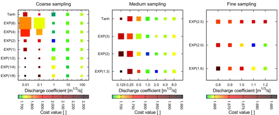
optimal than the exponential inflow scheme. The most ro-bust results are found for large exponents of the exponen-tial inflow scheme and a low discharge coefficient (Fig. 4, left). However, the cost value is quite high indicating that all simulations agree that this parameter combination lead to a decreased model skill. The lowest cost value (1.67) is found for an inflow exponent z=2 and a discharge coef-ficient c=1 m1/3s−1. At this point, the robustness of the result is still reasonable (σ =0.05). Two more refinements around this point were done. The medium sampling resolu-tion showed the lowest cost value (1.66) atz=1.33 andc=

2.0 m1/3s−1but a slight decrease in robustness (σ=0.06). Eventually, the best results were found in the fine resolution sampling forz=2 andc=1.1 m1/3s−1with a cost value of 1.66 andσ=0.05.

Next, the slope sensitivityκ was optimised. As κ is di-rectly included in the dynamical wetland extent calculation, wetland observations cannot be prescribed during this opti-misation step. However, the optimised values forzandcare now used in the model and give optimal constrains for the water balance calculation. Furthermore, a set of optimised simulations with static wetland extent is available from the first optimisation step. As two model simulations are better comparable to each other than to observations, we now use their simulated river discharge as optimisation target. Thus, we know that all differences between the river discharge curves are solely caused by the parametrization of κ and model deficits like the neglect of human impacts, already ex-isting model parameterizations or effects of model resolution have no effect on the analysis. Consequently, the analysis of river discharge differences is not limited to peak flow month and seasonality anymore. Instead, the normalized root mean square error (NRMSE) was calculated between the optimised river discharge with prescribed wetland extent and a series of 20 MPI-HM simulations with systematically variedκ. Start-ing with large values forκthe decrease infwweighted

aver-age NRMSE levelled off atκ=1. As no further simulation improvement was achieved with values ofκ <1, this value was accepted as optimalκat this model resolution.

As final step of the optimisation, it was investigated whether the MPI-HM with optimised wetland parameters is able to simulate river discharge in a better way than a MPI-HM control simulation without any wetland representation. Again, we applied the cost function (see Eq. 11) to com-pare the climatologies of simulated river discharge with the observed river discharge from the GRDC. For most catch-ments, the change in simulation error ranges within−8 % and 2 % with extremes up to −45 % and 61 %. No signifi-cant correlation of model improvement with the catchment’s simulated wetland fraction or area is found. However, the strongest influence of the DWES is evident for rivers with a large catchment and a mean simulated wetland area greater than 1000 km2. Discharge representations of rivers like Ama-zon and Ob are usually closer to observations in terms of peak flow month and seasonality than smaller catchments.

However, other large catchments, e.g. Mackenzie and Mis-sissippi are simulated with less agreement. On average, there is only a small improvement of the discharge simulation. On the one hand this is indicating that the restriction to global pa-rameters does not account for the vast diversity of different wetland types. Thus, it might be necessary to develop more specific parameters for different catchments in future model versions. On the other hand, we found no strong changes in artificially influenced river catchments like Nile, Amu Darya and Rhine, which are either used for irrigation or are strongly regulated. Human influences are not captured by the MPI-HM and therefore river discharge in those catchments cannot be simulated correctly. Here, the application of global param-eters prevents the MPI-HM from counteracting simulation errors that are not connected to wetlands. Thus, a thorough model evaluation is necessary to investigate whether the mi-nor improvement in river discharge can sufficiently constrain the wetland parameter optimisation and, thus, yield a satisfy-ing representation of the large scale wetland distribution.

3 Model evaluation

In order to evaluate the DWES, its results are compared to global observations of wetland extent and their seasonality. The analyses are mostly focused on large scale structures. Additionally, the representation of water bodies at grid cell scale is investigated to learn about the limitations of the DWES. Similar to the optimisation procedure, the MPI-HM uses the Watch Forcing Data (Weedon et al., 2011) from 1958–1999 as climate forcing for the evaluation simulations. Due to model spin-up, only the years 1963–1999 are consid-ered in the evaluation.

3.1 Global wetland distribution

Starting with the global scale analysis, we compare the sim-ulated wetland fraction with four datasets of global wetland and inundation observations. While these datasets have al-ready been used as boundary conditions in the optimisation procedure, the MPI-HM is not calibrated to match them. Thus, they can still be applied as an independent basis for the evaluation. However, it has to be noted that the obser-vations are not directly comparable to our simulation results as well as between one another because of the different wet-land definitions which they are based on. Thus, we first will provide some more details about the observation datasets.

Fig. 4. Optimisation results for MPI-HM simulations with prescribed wetland extent. The color indicates the skill of the simulation in respect

to river discharge observations (low values are best) and the size of the square indicates its robustness (inverse standard deviation, large squares are most robust). The sampling of parameter space of discharge coefficient and inflow parametrization is gradually refined from left to right.

The Land Surface Parameter set 2 (LSP2) was compiled by Hagemann et al. (1999) and revised by Hagemann (2002). It includes lakes as well as wetlands, and it is derived from the Global Land Cover Characteristics Data Base (US Ge-ological Survey, 2001), which was generated using satellite data with a resolution of 1 km. While lakes are easily iden-tified, the authors stated an increased uncertainty in the dis-tribution and extent of the wetland fraction. Lehner and D¨oll (2004) combined several existing maps and data bases into the Global Lake and Wetland Database (GLWD). It provides the maximum extent of lakes, reservoirs, rivers and wetlands at a resolution of 3000divided into 12 classes. Finally, a pure satellite product is taken into account which represents sur-face water covered areas on a monthly basis (Prigent et al., 2001, 2007; Papa et al., 2010). The satellite derived inun-dation dataset (SIND) is based on a 12 yr time series origi-nating from different satellites using active and passive mi-crowave measurements as well as visible and near-infrared imagery. From this data Prigent et al. (2001, 2007) and Papa et al. (2010) calculated inundated area fractions for 0.25° grid cells. While the authors claim that their multi-satellite ap-proach accounts for open water even under dense canopy, snow covered areas were masked out to avoid any confu-sion between open water and snow pack. All datasets are displayed in the upper and middle panels of Fig. 5.

The GLWD, LSP2 and MATT include no information about seasonal variations in wetland distribution, but provide their maximum observed extent only. Thus, the maximum climatological extent of the MPI-HM results and the SIND observation had to be computed prior to the analysis. Table 1 gives an overview about the simulated and the observed wet-land cover fractions for every continent. In all regions except Asia, the largest wetland fraction estimate is produced by

the MPI-HM. It strongly overestimates the wetland extent for South America and Africa (27.5 % and 10.1 %, respectively) compared to the observations. However, for North Amer-ica the GLWD indAmer-icates a similar extensive wetland cover as the MPI-HM (around 18.1 %) and also agrees well for Asia (6.1 %). For Europe, a wetland extent of 8.3 % is sim-ulated which is close to the estimate of the MATT dataset. With 4.3 % coverage, the Australian wetland extent is sim-ulated about 1 % larger than seen in the GLWD. Globally, the MPI-HM simulates a wetland fraction of about 12 %, fol-lowed by the GLWD with 8.1 %. Table 1 also gives informa-tion about the large variainforma-tions in the wetland observainforma-tions. For North and South America the GLWD indicate a 3 times larger wetland cover than the MATT and LSP2, respectively. Also on global scale, the estimates range from 3.7 % (MATT) to 8.1 % (GLWD) and thus demonstrate the large uncertainty in observations.

Fig. 5. Observed (top, middle) and simulated (bottom) maximum wetland distribution. The colors indicate the wetland fraction for every

0.5◦grid cell. The black boxes highlight regions of pronounced wetland occurrence.

Table 1. Simulated and observed maximal wetland cover for different continents in percent of the global land surface without Antarctica.

Continent MPI-HM GLWD LSP2 MATT SIND

North America 18.11 16.72 5.59 4.62 9.29 South America 27.46 9.25 2.23 3.86 6.23 Europa 8.31 4.55 4.18 7.40 5.84 Africa 10.13 5.11 1.49 2.34 2.54 Asia 6.13 6.98 9.34 3.53 7.82 Australia 4.32 3.14 0.27 2.14 2.20

Global 11.92 8.11 5.09 3.71 6.20

pattern as the observations. The best agreement is visible for North America where the pattern of wetland distribution is well matched. However, the maximum wetland extent ex-ceeds the range of observed values. The wetlands in the north of Europe are well represented and their extent is similar to the observations. Also the Siberian wetland regions are re-produced by the MPI-HM but especially the East Siberian wetland cluster is underestimated. Likewise, too few wet-lands are simulated for Southeastern Asia in China and the region between Vietnam and Myanmar if compared to the LSP2 and SIND. In contrast, the GLWD and MATT display less wetlands than the MPI-HM in this area. In the Southern Hemisphere the simulated wetlands concentrate in the Ama-zon and Congo catchments. While this location is generally confirmed by the observations, the overall extent is strongly

overestimated by the model. Overall, these simulation results demonstrate that the DWES is able to reproduce the large scale wetland patterns. Although there are differences in the extent of the wetland clusters, these differences are mostly in the same magnitude as the differences among the wetland observations themselves. However, the model fails to repre-sent a realistic wetland extent for the tropical parts of South America and Africa.

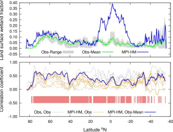
Fig. 6. Top: zonal means of land surface wetland fraction. The grey area indicates the range of the observation datasets, the green curve

shows their mean extent and the blue curve shows wetland fractions as simulated by the MPI-HM (blue). Bottom: zonal correlation between the MPI-HM wetland extent and the mean of observations (blue), between the MPI-HM wetland extent and the four observation datasets (orange) and between the observations themselves (grey). Displayed are running means over 2.5 latitudes. The red boxes indicate latitudes where the correlation significance level between the MPI-HM results and mean extent of the observations is above 95 %.

shape of the observation mean curve and is mostly found in the upper part of the observational range. Similar to the observations, the largest wetland fractions are computed be-tween 40◦ _{and 70}◦_{N. However, the second peak between} 10◦_{N and 20}◦_{S is overestimated by the MPI-HM by a} fac-tor of almost four compared to the observation mean. Further south, the simulated zonal mean wetland extent first drops to the range of observed values but shows a very noisy signal due to the small land surface fraction in these latitudes.

We also investigate the spatial agreement between simu-lation and observation. Figure 6 (bottom) shows the linear correlation coefficient of the wetland fractions along the lat-itudes for the different wetland fraction data. Considering first the correlation between the observation datasets them-selves, the coefficients lie mostly between 0 and 0.5. At some latitudes, e.g. between 40◦and 50◦N almost no corre-lation is seen, whereas at other latitudes some observational datasets are highly correlated. The noisy signals indicate that the agreement between the observations varies strongly from latitude to latitude and there is no combination of observa-tion datasets that show a high correlaobserva-tion over a larger lati-tude band. The figure also demonstrates that the correlation coefficients between simulation and observations lie in the same range as those between the observations. Focusing on the correlation between the simulation and the mean of the

observations, the highest correlation coefficient of about 0.5 is found for the high northern latitudes while the lowest relations concentrate directly south of the equator. The cor-relation is significant for the majority of latitudes.

3.2 Seasonal variations in wetland extent

Beside the simulation of maximum wetland extent, the vari-ation of wetland extent is another key aspect of our study. These variations are a measure for the response of the MPI-HM to changes in climatic forcing and its analysis shows whether the hydrological cycle of wetlands is represented in the MPI-HM in sufficient detail. However, long-term time series, about year to year variability in wetlands, are rare on a global scale. Furthermore, their amplitude is exceeded by the amplitude of seasonal variations in the MPI-HM simu-lations. Thus, we focus our analysis on seasonal variations rather than year to year changes. Concerning the model accu-racy and its high sensitivity to short-term climatic variations we argue that both are better demonstrated by the model’s representation of the seasonal wetland extent variations.

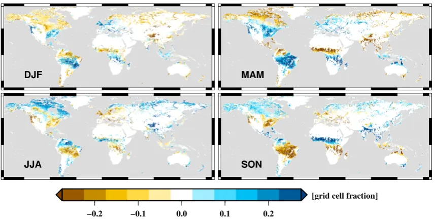
Fig. 7. Deviation of the wetland fraction from its yearly mean for all seasons as simulated by the MPI-HM.

the wetland fraction decreases during DJF. It subsequently increases again starting from the south during MAM and reaching the far north in JJA. This behaviour reflects the de-creased wetland inflow during the cold season and the in-creased inflow due to snowmelt. In the tropics the wetland extent follows the rainy and dry seasons which are caused by the movement of the Intertropical Convergence Zone. Con-sequentially, the MPI-HM computes decreased wetland tions north of the equator in DJF and increased wetland frac-tions south of it. This pattern is mirrored during JJA.

The model evaluation is restricted to one observational dataset, the SIND, because it is currently the only global dataset with monthly values of inundated area. Figure 8 dis-plays the climatologies of simulated and observed wetland extent for different latitude bands. For the high latitudes larger than 60◦, the MPI-HM simulates decreased wetland fractions during winter and a strong peak due to snowmelt in June. Furthermore, a second wetland extent maximum is visible for autumn. However, the SIND shows only a single peak and no wetlands during winter because satellites are not able to identify wetlands below snow cover. Thus, snow cov-ered grid cells have been masked out in the observational data (Papa et al., 2010). After applying the SIND snow mask for the simulated wetland fractions, both datasets agree well in the timing of the wetland extent variations. A similar effect is seen for the mid latitudes (between 23.5◦and 60◦) where the application of the snow mask results in a good agreement between simulated and observed wetland extent seasonality, too. In the low latitudes (less than 23.5◦) the snow mask has no significant effect on the simulation results. Here, the wet-land seasonality agrees mostly well with the SIND in timing as well as in the relative amplitude of the variations.

3.3 Results on grid cell scale

In order to learn about the limitations of the DWES, we also analyse the results on the scale of just a few grid cells. In this analysis we do not expect to represent the observed wetland fractions perfectly but to learn under which conditions the model succeeds or fails on the grid cell scale.

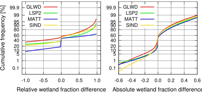
First, we focus on the differences between the maximum MPI-HM wetland fraction and the observation datasets. In order to increase the robustness of the analysis, an aver-age wetland extent is calculated for every grid cell based on the grid cell itself and its 8 neighbouring grid cells. Thus, the data is smoothed and spatial offsets of just one grid cell are neglected. The relative difference is calculated as fw,sim−fw,obs/ fw,sim+fw,obs and displayed in Fig. 9

Fig. 8. Seasonality of wetland extent relative to its maximum for

different latitude bands. The green color indicates the SIND obser-vations, the blue the MPI-HM results and the yellow line represents the MPI-HM results corrected with the snow mask. For low latitudes the yellow curve lies on top of the blue because the snow mask has no significant impact on the wetland fraction in these regions. The shaded areas indicate the standard deviation.

of absolute differences cumulative frequency (see Fig. 9, right), the steepest step (about 55 % of all grid cells) oc-curs for wetland fraction differences around zero. Again, all dry regions are included in this peak but also most of the ar-eas where either MPI-HM or observations indicate wetlands. This demonstrates that the large relative differences are often related to very small absolute differences. The absolute dif-ferences of the remaining grid cells are more often positive than negative, indicating that the MPI-HM more often over-estimates wetland extent than underestimating it. For the rel-ative as well as the absolute differences, these results are sim-ilar if the observation datasets are compared to each other in-stead to the MPI-HM results. Testing the correlation between the grid cell wetland fractions we find that the MPI-HM wet-land fractions correlates significantly but weakly with the observation. The correlation coefficient spreads from 0.20 (MATT) to 0.44 (GLWD). This is in the same range as the observations correlate with each other. The minimum cor-relation coefficient between observations is 0.12 (LSP2 and MATT) and the maximum lies at 0.50 (GLWD and MATT).

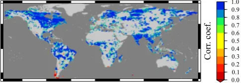
Second, we enhance the analysis of seasonal variations by calculating the temporal correlation between simulation and observation (Fig. 10) for every grid cell. Similar to the first analysis, we use a 9 grid cell average as basis for the corre-lation. Additionally, the snow mask is applied. For most of

the large scale wetland clusters, a good temporal correlation is achieved, but in between those areas pronounced regions of insignificant correlations are found. Examples for these regions are wide parts of Europe as well as some areas in South America, Africa and Australia. Additionally, insignifi-cant correlations occur north of 60◦N. Investigating the rea-sons for this pattern, we find a strong impact of the snow mask. As its application decreases the number of months that can be used in the correlation analysis, the correlation becomes less significant. Occasionally, the significance is bi-ased towards higher values for larger wetlands. However, the latter feature is not a robust result. Neglecting all insignif-icant correlations, a global mean correlation coefficient of 0.70 is computed.

Additionally, in reference to the variations of wetland ex-tent, variations in wetland water level are also an important indicator of model quality. However, long-term time series of wetland water level exist only for very few locations and are often interrupted during winter. Thus, we use satellite ob-served lake level data as a substitute for wetland observa-tions. While the MPI-HM does not simulate lakes explicitly, they are included in our definition of wetlands (see Sect. 2.3). Of course, lake level data accounts only for a small part of the simulated surface water. Thus, we restrict our analysis on the correlation of simulated and observed seasonality in the water levels. For this analysis, we assume the observed lake level variations to be representative for all surface wa-ter bodies within a grid cell size area, because two of their major water sources, rainfall and inflow from upstream ar-eas, are often the same for both water bodies. We also com-pare the overall range of variability in observed lakes and simulated wetlands, but only to learn about the limitations of the DWES. The Global Reservoir and Lake Monitor (GRLM, 2011) provides data on lake level variations collected by sev-eral satellites. In our analysis we used data for 79 lakes for the period between 1992 and 2002. Figure 11 displays the linear correlation coefficient between the observed and sim-ulated monthly climatologies of water level variations for 79 lakes. For 12 lakes no surface water occurs in the model and 27 lakes do not show any significant correlation above the 90 % confidence level. For 24 lakes the observation corre-late very well with the simulation with coefficients above 0.8. The correlation of another 14 lakes is at least 0.5 while the remaining three lakes show a significant negative correlation. Investigating the reasons for the insignificant correlations, we find that insignificant results occur preferably for lakes with a mean simulated water throughflow below 300 m3s−1_.

Fig. 9. Cumulative distributions of relative (left) and absolute (right) wetland extent difference at grid cell scale between the MPI-HM

simulation and observations.

this model behaviour, we find good agreements only for those lakes which have a low variability in the observations or are simulated with a large grid cell fraction. In these cases, the water throughflow does not play any significant role.

4 Discussion

In terms of large scale patterns, the DWES represents the wetland distribution successfully. However, deficits in com-putation of the wetland extent have been revealed during the evaluation and need to be discussed. Another important ques-tion is how the representaques-tion of wetlands in the MPI-HM might affect hydrological components in the climate system, e.g. due to enhanced ET. As our study is conducted using a global hydrological model with prescribed climatic forcing, we cannot directly investigate any large scale hydrological feedbacks of wetlands. Still, we can evaluate whether wet-lands have the potential to impact the land surface hydrology significantly.

4.1 Wetland impact on ET and runoff

There are a number of possibilities how wetlands might in-fluence the Earth system. Several studies focus on changes in atmospheric methane concentration (e.g. Gedney et al., 2004; Finkelstein and Cowling, 2011) and its effect on mean sur-face temperature as a result of the change in radiative forc-ing. Coe and Bonan (1997) simulated the influence of surface water on Mid-Holocene climate conditions and found an in-crease in net surface radiation, latent heat and humidity as well as an decrease in the sensible heat flux. These changes lead to a cooling of the atmosphere and an alteration of the atmospheric flows resulting in changes in the regional precip-itation patterns. Dadson et al. (2010) and Taylor (2010) con-centrated on the Niger inland delta. The authors related the seasonal inundation in this region with enhanced evaporation and an increase in cloud cover and convection. In our study

we concentrate on the impact of wetlands on ET and runoff. Here, we compare the results of a MPI-HM simulation us-ing the DWES to a MPI-HM control simulation without any wetland representation.

In the MPI-HM, the only connection from wetlands to the atmosphere is via the ET. We find that the simulation of wet-lands increases the annual ET by 4.5 mm on average over the global land surface without Antarctica. The largest ET increase occurs during the summer months. For most of the land surface, this ET anomaly is below 0.1 mm d−1_.

How-ever, regionally much stronger effects occur, for instance, in high latitudes of North America and Eastern Siberia. Due to open water in the simulated wetlands, they almost evapo-rate at the potential evapo-rate resulting in ET anomalies exceeding 1.0 mm d−1(≈25 %) during the summer months. In contrast, small negative ET anomalies are simulated during dry spells for some grid cells in equatorial regions. This effect is related to a technical issue in the model. In contrast to the land sur-face, the wetland fraction is simulated without any canopy storage because its ET is already at maximum as long as sur-face water exists. In some cases, the open water sursur-faces may vanish completely during the summer resulting in decreased ET. ET does not reach its maximum value, before the soil is saturated again. While soil moisture is similarly low in the control simulation, its canopy storage reacts much faster to precipitation events and may allow for short-term high ET responses. However, this effect occurs only sporadically and does not effect the overall ET increase significantly.

Fig. 10. Correlation coefficient of the temporal correlation between

SIND and MPI-HM wetland extent climatologies. Only correlation with a significance higher than 90 % are shown.

with a lower hydraulic conductivity. In spite of this, a pos-itive drainage anomaly is found in wetland regions that are dominated by river flows. In the MPI-HM control version, water that once entered the river routing scheme is not avail-able to the land surface anymore but flows directly into the ocean via the river network. However, the DWES allows for the recharge of wetlands by river flow and thus ET and drainage can be increased in downstream grid cells. Conclu-sively, the increase in drainage is not so much a result of the wetland simulation but rather enabled by the coupling between the horizontal and vertical water flows. Although positive drainage anomalies are just around 0.2 mm d−1, they partly contribute to an increase of river flow in some catch-ments (see Sect. 4.2).

After the spin-up phase of the model, the DWES has no strong impact on the water storages of the MPI-HM. The changes in snow water equivalent, skin reservoir and aver-age soil moisture content are below 0.01 mm a−1_{. The only}

storage that shows a trend in its content is the surface water storage. During the simulation period, its average increase is about 0.15 mm a−1.

4.2 Wetland impact on river discharge

Focusing on a selection of about 96 major river catchments, we find that almost all of them are sensitive to changes in wetland extent. In most cases, the simulated mean river dis-charge decreases in the presence of wetlands. Most catch-ments only experience a small decrease up to 5 % of the an-nual discharge but also large changes up to 25 % decrease oc-cur. Similar effects are also apparent in the discharge season-ality. Comparing the variance of river discharge, the majority of catchments reveals a decrease between 0 % and 45 % with a maximum decrease of 90 %. Additionally, the peak flow is delayed when the DWES was active. For most catchments this delay is less than one month. These changes can be ex-plained with the additional wetland water reservoir and its outflow parametrization. Due to its longer retention time (see Sect. 2) water release from the wetland reservoir is slower than from the river reservoir. Thus, the flow peak is decom-posed in a fast and a slow component. The main peak is de-layed until the superposition of both components reaches its

Fig. 11. Map of correlation coefficients in lake level climatologies

between the MPI-HM simulation and GRLM observation. Light grey points indicate insignificant correlations and dark grey points indicate locations where no surface water body was simulated by the MPI-HM.

maximum. Additionally, the variation in river flow decreases because the wetland reservoir stores peak flow water and re-leases it after the flood event. In contrast, the overall decrease in river flow occurs due to the interactive coupling between the vertical and horizontal water balance sub-models. In this MPI-HM setup, water that is stored in the wetland reservoir is able to evaporate thereby reducing river discharge. These processes are also reported for most observed wetlands (Bul-lock and Acreman, 2003).

About seven catchments show the opposite reaction to the presence of wetlands. Increased mean flow and seasonality are evident in these catchments but no earlier peak flows can be recognized. The strongest increases are up to 20 % for the mean flow and up to 40 % for the seasonal variations. Ex-amples for these exceptions are the catchments of the Blue Nile, the Sao Francisco and the Colorado River. They are located in regions where either wetlands are simulated with a large extent and a considerable water turnover or steep slope conditions prevail that facilitate fast water transport. In these catchments, water is transported more efficiently in the wetlands than via overlandflow. Together with the posi-tive drainage anomaly, the bypass of overland flow causes lo-cally increased river discharge. This behaviour is confirmed by Bullock and Acreman (2003) who reported on similar ob-servations in some headwater wetlands.

In summary, about 530 km3a−1 less water reach the oceans than in the control simulation. This decrease balances most of the ET increase of 670 km3a−1. As the inflow de-cline is just about 1 % of the overall simulated ocean inflow, we do not expect any significant influence on the ocean in terms of hydrology. However, the decline might have impli-cations for the nutrient or sediment transport into the ocean.

4.3 Limitations of the DWES

definition or the application of a general approach for dif-ferent wetland types.

The most obvious deficit in the MPI-HM is its strong over-estimation of tropical wetland extent. For this region, Figs. 5 and 6 indicate an about four times larger wetland extent in the MPI-HM than stated in all four observation datasets. It is obvious that in the model too much water is available on the land surface indicating either a wet bias in the precip-itation forcing, a too low PET or too low horizontal out-flow from the respective basins. Precipitation and PET are part of the prescribed climate forcing. While precipitation is directly included in the WFD, PET is computed based on the Penman-Monteith equation for reference ET using me-teorological variables of the WFD. Following Weedon et al. (2011), globally constant parameters with the values for short grass were used for the vegetation height and the surface re-sistance. However, the major land cover type in these areas is tropical forest. As Amazonian rainforest usually has a sig-nificantly higher ET than grassland (e.g. Costa and Foley, 1997; von Randow et al., 2004), PET is probably underesti-mated by the model leading to too extensive wetlands. Ad-ditionally, too low outflow could cause the cumulation of surface water and indicate an inability of the DWES to ac-count for the specific wetland types in these regions. While the LSP2 and SIND do not contain any information on wet-land types, these wetwet-lands are classified as floodplains and swamp/flooded forests in the GLWD as well as forested and non-forest swamps in the MATT. In both maps these types occur most often in the tropics and are related to seasonal flooding. Thus, the overestimated tropical wetlands indeed belong to a certain wetland group. This fact gives rise to the assumption that the DWES might not be able to account for seasonal inundation or other floodplain processes in a realis-tic way. However, in comparison to the GRDC data, the peak flows of the Amazon and Congo catchments are simulated very well but the overall river discharge is already exceeding the observed values. A further increase in outflow velocity would lead to earlier peaks and increasing river discharge and thus decrease the model skill. Alternatively, the excess surface water could be related to an underestimation of soil storage capacity. In the MPI-HM the soil storage capacity is prescribed by the plant root depth. However, the real soil depth to the bedrock could exceed the root depth by some extent and store a considerable amount of the surface water. For these reasons, we assume that the PET computation or the soil bucket parametrization are causing the wetland over-estimation rather than the DWES.

Compared to the LSP2 and SIND, the MPI-HM underesti-mates the wetland extent in Southeastern Asia. Both observa-tion datasets are based on satellite products, which indicate the existence of surface water. These wetlands are not re-ported by the GLWD and MATT. Indeed, extensive wetlands exist in this region but these are mostly artificially formed (Mudge and Adger, 1995), e.g. due to irrigation. They are not captured by the model because the MPI-HM does not

account for human impacts. The extent overestimation in the Eastern USA and Western Europe compared to the LSP2 and SIND can be attributed to the same shortcoming albeit in the opposite way. In these regions, existing wetlands were artifi-cially drained (Finlayson and Davidson, 1999). Some regions lost more than 50 % of their wetland area, e.g. the south-western part of the USA (Dahl and Allord, 1996). However, these wetland losses were mainly caused by human impact rather than by climate change and are therefore not capture by the model. Instead, the DWES represents potential wet-lands which could be sustained by climate conditions but were removed by landscape management.

Finally, the Siberian wetlands are underestimated com-pared to all observations. The underestimation is strongest for the GLWD and MATT and less pronounced for the LSP2 and SIND. This indicates that not all of the wetlands have surface water. Indeed, peatlands, which are most common in the high northern latitudes, are often waterlogged but not necessarily inundated. While water logged conditions are considered in the water balance calculations of the DWES, the wetland extent calculation requires surface water to com-pute any surface water changes (see Sect. 2.2). Conclusively, the DWES neglects most peatlands causing a general under-estimation of wetland extent in the respective areas.

A major point of interest is the MPI-HM’s skill to repre-sent wetlands on grid cell scale. While seasonality of wetland extent and their water level variation are simulated with some confidence, the maximum wetland extent as well as the mag-nitude of lake level variations differ from observed values. In order to explore the reasons for these model deficits, the rela-tion of the differences to a number of other model variables were investigated. Concerning the differences in maximum wetland extent, we find that they as well as their standard de-viations are low for small simulated wetlands extent. Both increase for a larger wetland fraction and a larger overall wa-ter turnover. Obviously, the MPI-HM is betwa-ter in identifying areas not suitable for wetland formation than in estimating the exact extent of wetlands that form in the remaining ar-eas. Furthermore, the differences also depend on whether the wetland is dominated by vertical or horizontal water flows. Wetlands that are sustained mainly by horizontal flows are simulated too large by about 15 % to 30 % of grid cell area, whereas wetlands with predominantly vertical flows are sim-ulated too little by about 0 % to 5 % grid cell area. Also, the standard deviation of about 0.3 in the first case is reduced to 0.1 in the second case. Decomposing the water flows into inflows and outflows, both flow components show a similar behaviour, although for the inflows, the decline in difference and standard deviation occurs not before the overall water flow comprises about 80 % vertical flows. Finally, the dif-ferences are compared to the size of the upstream area for every wetland grid cell but no systematic bias is evident in this relation.