Technical Note: Bias correcting climate model simulated daily temperature extremes with quantile mapping

temperature extremes with quantile mapping

B. Thrasher1,2, E. P. Maurer3, C. McKellar4, and P. B. Duffy5 1_{Climate Analytics Group, Palo Alto, CA 94303, USA}

2_{Climate Central, Princeton, NJ 08542, USA}

3_{Santa Clara University, Civil Engineering Dept., Santa Clara, California, 95053-0563, USA} 4_{San Jose State University, Dept. of Meteorology and Climate Science, San Jose, CA 95126, USA} 5_{Lawrence Livermore National Laboratory, Livermore, CA 94550, USA}

Correspondence to: B. Thrasher ([email protected])

Received: 27 March 2012 – Published in Hydrol. Earth Syst. Sci. Discuss.: 25 April 2012 Revised: 16 August 2012 – Accepted: 20 August 2012 – Published: 17 September 2012

Abstract. When applying a quantile mapping-based bias cor-rection to daily temperature extremes simulated by a global climate model (GCM), the transformed values of maximum and minimum temperatures are changed, and the diurnal temperature range (DTR) can become physically unrealistic. While causes are not thoroughly explored, there is a strong relationship between GCM biases in snow albedo feedback during snowmelt and bias correction resulting in unrealistic DTR values. We propose a technique to bias correct DTR, based on comparing observations and GCM historic simu-lations, and combine that with either bias correcting daily maximum temperatures and calculating daily minimum tem-peratures or vice versa. By basing the bias correction on a base period of 1961–1980 and validating it during a test pe-riod of 1981–1999, we show that bias correcting DTR and maximum daily temperature can produce more accurate es-timations of daily temperature extremes while avoiding the pathological cases of unrealistic DTR values.

1 Introduction

While monthly, seasonal, and annual changes in climate have the potential to affect ecosystems and human development (e.g., Fowler and Kilsby, 2003; Palmer and Raisanen, 2002; Schneider et al., 2007), there has been an increasing inter-est in the effect of shorter-term extreme events (Christensen et al., 2007; IPCC, 2011). These events can cause billions of dollars (USD) in damages in hours or days (Bouwer and

Vellinga, 2003), and changes in their magnitude and/or fre-quency are projected to increase the risk of amplified dam-ages in future decades (Easterling et al., 2000).

To assess regional changes in daily extreme rainfall and temperature, global climate model (GCM) output must be downscaled to a more regionally appropriate scale. The many methods to achieve this can be broadly classified as dy-namical, which uses a fine-scale climate model to interpo-late GCM signals, and statistical, which uses historically de-rived statistical relationships between GCM-scale and fine-scale features to estimate regional climate (Christensen et al., 2007). In either case, before any downscaled data can be ingested into a model to estimate specific impacts of cli-mate change, some adjustment to account for the GCM bi-ases must be included, since at least some of the bias is sys-tematic, being induced by factors such as inadequate terrain resolution in the GCM (Haerter et al., 2011).

3310 B. Thrasher et al.: Bias correcting climate model simulated daily temperature

Fig. 1. For Case 1, the total number of occurrences for the validation

period of 1981–1999 whereTmin> Tmaxafter BC. Results for two

GCM simulations are shown: a high number of occurrences (upper panel) and a low number of occurrences (lower panel).

temperature (Tmax) and minimum daily temperature (Tmin)

are adjusted with quantile-mapping bias correction (here-inafter referred to as BC), the bias correction can modify the diurnal temperature range (DTR) and in some instances can result in the relationship betweenTmaxandTminbeing

phys-ically unrealistic. In this study, we compare the different al-ternatives to (1) minimize the error in the bias-correctedTmax

andTminvalues, and (2) reduce the frequency of cases where

TmaxandTmin are reversed in the BC process. We examine

the ability to minimize these instances by instead applying the BC to diurnal temperature range (DTR) and eitherTmin

orTmax, where the remaining variable is derived by adding

or subtracting the DTR as appropriate. In this way GCM-simulated trends in DTR,TminandTmaxcan be retained

with-out the need for ad hoc adjustments.

2 Methods and data

Table 1 lists the 17 GCM simulations from which daily

Tmax and Tmin values were obtained for the 1961–1999

period. These GCM simulations were archived as part of the World Climate Research Programme’s (WCRP’s) Coupled Model Intercomparison Project phase 3 (CMIP3)

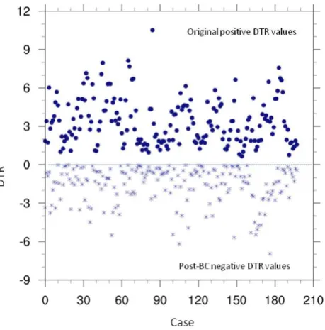
Fig. 2. Cases whereTmin> Tmaxat the grid cell at 57◦N, 43◦E,

during 1980–1989 for GCM run MRI Run 3.

multi-model dataset effort (Meehl et al., 2007). GCM out-put was interpolated onto a common 2-degree grid to enable intercomparison and summaries across GCMs. For an obser-vational baseline, a 0.5-degree daily global gridded dataset (Adam and Lettenmaier, 2003; Maurer et al., 2009) was ag-gregated to the same 2-degree grid spacing. DTR was calcu-lated for each day in the 39-yr GCM simulations, as well as for the gridded observations, as the difference betweenTmax

andTmin.

The BC approach used here is essentially that of Mau-rer et al. (2010), but, rather than being applied to daily av-erage temperatures, it is applied toTmax,Tmin, or DTR

in-dependently. In summary, the BC uses a base period where both daily observations and daily GCM-simulated values are available. For each day of the year, a moving window of

±15 days is used to select all candidate days representative of the date, and all of these candidate days are sorted and ranked to produce for each calendar day two cumulative dis-tribution functions (CDFs): one for observations and one for the GCM. For this study, we used 1961–1980 as the base period for which the BC relationships were derived. Thus for any calendar date, there would be 31 days in the mov-ing window and 20 yr in the base period, resultmov-ing in 620 points to define the CDF for each variable. A bias-corrected value for a GCM-simulated daily value is retrieved by using the CDF for the GCM to determine the quantile associated with the value, and then drawing the observed value from that same day’s CDF for the same quantile. For example, a medianTmaxvalue for 15 February in the GCM output will be

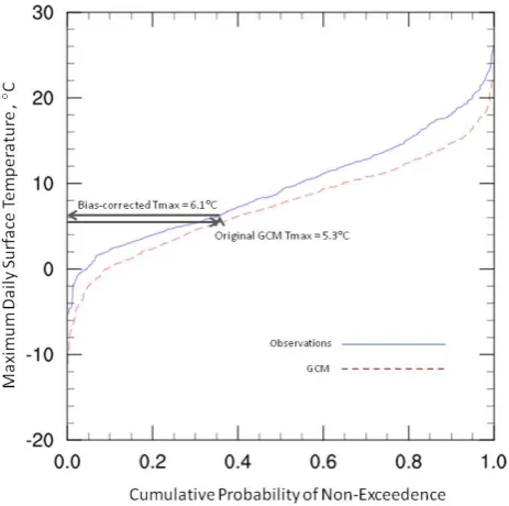
Fig. 3. CDFs for maximum daily temperature based on the period

1961–1980 for observations and MRI Run 3. Arrows illustrate the quantile mapping for the dailyTmaxvalue for 17 April 1983.

for 15 February, where the median value is that daily value exceeded 50 % of the time in the set of 620 days defining the CDFs for 15 February.

We perform three variations of daily temperature BC: – Case 1: BC performed forTmaxandTmin;

– Case 2: BC performed forTminand DTR, withTmax

cal-culated asTmin+ DTR;

– Case 3: BC performed forTmaxand DTR, withTmin

cal-culated asTmax−DTR.

Case 1 is the default case, with shortcomings discussed above. Cases 2 and 3 are evaluated by comparing the root-mean-square error (RMSE) across all days and grid cells for global land areas, where the RMSE is calculated for the de-rived variable (i.e., for Case 2 RMSE forTmax is assessed,

and for Case 3 RMSE forTminis assessed). The three cases

are assessed for the validation period of 1981–1999.

3 Results and discussion

The results for Case 1 are shown in Fig. 1. Despite the wide variability in the number of cases where Tmin> Tmax after

BC of the GCM output, Fig. 1 shows, for extreme high and low cases, that these tend to occur predominantly at high lat-itudes (and this is generally the case for all of the GCM sim-ulations used in this study). For these high latitude regions, the GCMs have biases in mean and/or variability that tend to produce more occurrences ofTmin> Tmaxwhen adjusted

Fig. 4. Same as Fig. 3, but for minimum daily temperatures.

Table 1. GCMs and run numbers included in this study.

Simulation

1 CCCMA-CGCM3-1: Run 1 2 CCCMA-CGCM3-1: Run 2 3 CCCMA-CGCM3-1: Run 3

4 CNRM-CM3

5 GFDL-CM2-0 6 GFDL-CM2-1 7 IPSL-CM4

8 MIROC3-2-MEDRES: Run 1 9 MIROC3-2-MEDRES: Run 2 10 MIUB-ECHO-G: Run 1 11 MIUB-ECHO-G: Run 2 12 MIUB-ECHO-G: Run 3 13 MPI-ECHAM5

14 MRI-CGCM2.3.2A: Run 1 15 MRI-CGCM2.3.2A: Run 2 16 MRI-CGCM2.3.2A: Run 3 17 MRI-CGCM2.3.2A: Run 4

through BC. How this can occur is demonstrated here using a single grid cell located at latitude 57◦_{N longitude 43}◦_E (northeast of Moscow, Russia) from MRI Run 3 (Run 13 in Table 1). For the decade of the 1980s, 3653 days in total, there were 198 cases where the bias correction resulted in

Tmin> Tmax, which are depicted in Fig. 2. For this decade, the

3312 B. Thrasher et al.: Bias correcting climate model simulated daily temperature

Fig. 5. Fraction of occurrences across all (land area) GCM grid cells

and all March–May days in the validation period of 1981–1999 versus the snow albedo feedback error, calculated from Hall and Qu (2006) based on GCM-simulated seasonal cycle between April and May.

Fig. 6. The RMSE (◦C) between gridded observations and three versions ofTmax for 17 GCM simulations: regridded daily GCM Tmax(blue), bias-corrected daily GCMTmax(red), and dailyTmax

derived from bias-corrected DTR andTmin(green, Case 2).

cases with small DTR, relative to the GCM bias, are more prone to having this issue.

The method by which this occurs is illustrated for the same grid cell and run used above for one of the cases in Fig. 2, corresponding to 17 April 1983. The CDF for maximum tem-perature is constructed as described above, using a window of±15 days around 17 April. Using the period 1961–1980 as the climatological period, 620 days are used to define the CDFs. As shown in Fig. 3, the GCM underpredicts the daily

Tmaxvalue throughout the distribution. Figure 4 shows the

same as Fig. 3, but forTmin, which the GCM also

underesti-mates, but by a much wider margin than forTmax. The

quan-tile mapping is illustrated in Figs. 3 and 4, transforming the raw GCMTmaxandTminof 5.3◦C and 1.9◦C, respectively,

Fig. 7. The RMSE (◦C) between gridded observations and three versions ofTmin for 17 GCM simulations: regridded daily GCM Tmin(blue), bias-corrected daily GCMTmin(red), and dailyTmin

derived from bias-corrected DTR andTmax(green, Case 3).

Fig. 8. RMSE (◦C) between gridded observations and two versions of DTR for 17 GCM simulations: regridded daily GCM DTR (blue) and bias-corrected daily GCM DTR (red).

to bias-corrected values of 6.1◦C and 11.6◦C, respectively, producingTmin> Tmaxand a physically impossible DTR.

termined. It should be noted that, even in the extreme case over Eastern Europe for the worst case of the GCMs used here, fewer than 400 occurrences are observed in the 19 yr validation period, indicating less than 6 % of days having

Tmin> Tmax, with most of global land areas and GCM

simu-lations exhibiting far less than this. On average for all GCM simulations,Tmin> Tmaxoccurs approximately 0.25 % of the

time.

The two approaches conducted in this study to remedy the occurrence ofTmin> Tmaxfollowing the BC process, Cases 2

and 3, are compared to determine the preferable alternative. Figure 6 shows the results for Case 2, where the “obs vs. original BC” RMSE refers toTmax produced as in Case 1,

and the “obs vs. derived BC” being that calculated as de-scribed above for Case 2. First, both cases of bias correction improve the original GCM output, as is evident by the RMSE for both Case 1 and Case 2 being lower than for the “obs vs. GCM” points. The RMSE shown in Fig. 6 for Case 2 is higher than for Case 1, which shows that, for all GCM simulations, the approach of Case 2, while eliminating oc-currences ofTmin> Tmax, deteriorates the estimation ofTmax

in the BC process.

Figure 7 shows similar results to Fig. 6 but for Case 3. In this alternative, “obs vs. original BC” refers to the BCTmin

as in Case 1, and “obs vs. derived BC” is that calculated ac-cording to the description of Case 3 above. As with Case 2 (Fig. 6) for most GCMs, either approach to BC (Case 1 or Case 3 in Fig. 7) results in decreased RMSE, thus producing

Tminvalues that bear greater resemblance to observations. In

contrast to Case 2, theTminvalues derived in Case 3 show

reduced RMSE for 12 of the 17 GCM simulations, indicat-ing that this alternative not only removes the possibility of

Tmin> Tmax in the BC process, but results in an improved

estimation ofTminon average.

That GCM-simulatedTmaxappears more capable of

ben-efiting from a quantile mapping bias correction than Tmin

suggests that the biases, relative to observations, exhibited forTmaxmay be more systematic than those forTmin. While

a mechanism explaining this has neither been expressed in the literature, to the authors’ knowledge, nor been proposed here, the consistency with other research results (Maurer et al., 2012) is encouraging as a topic for future efforts.

Finally, while Case 3 appears to be the best solution of the alternatives assessed in this study, since applying BC to DTR

We evaluated the potential to improve the quantile mapping bias correction approach when applied to daily GCM output of maximum and minimum temperatures. A direct bias cor-rection of both TmaxandTminresults in some cases where

the unrealistic occurrence ofTmin>Tmaxappears. To remedy

this, we first derive the diurnal temperature range for each day, and then apply the bias correction to DTR and either

TmaxorTmin, calculating the remaining variable.

We find that bias correcting daily DTR and Tmax and

calculatingTminas Tmax-DTR eliminates the occurrence of

Tmin> Tmaxand in general improves the estimation ofTmin

compared to bias correctingTmindirectly. This approach will

be further assessed and implemented in future applications of quantile mapping bias correction of daily GCM temperature output.

Acknowledgements. Funding for this work was provided by the U.S. Army Corps of Engineers under grant W912HQ-IWR-CLIMATE. We acknowledge the modeling groups, the Program for Climate Model Diagnosis and Intercomparison (PCMDI) and the WCRP’s Working Group on Coupled Modelling (WGCM) for their roles in making available the WCRP CMIP3 multi-model dataset. Support of this dataset is provided by the Office of Science, US Department of Energy.

Edited by: B. Schaefli

References

Abatzoglou, J. T. and Brown, T. J.: A comparison of statistical downscaling methods suited for wildfire applications, Int. J. Cli-matol., 32, 772–780, doi:10.1002/joc.2312, 2012.

Adam, J. C. and Lettenmaier, D. P.: Adjustment of global gridded precipitation for systematic bias, J. Geophys Res., 108, 1–14, 2003.

Bouwer, L. and Vellinga, P.: Changing climate and increasing costs – Implications for liability and insurance Climatic Change: Im-plications for the Hydrological Cycle and for Water Manage-ment, edited by: Beniston, M., Advances in Global Change Re-search, Springer Netherlands, 429–444, 2003.

projec-3314 B. Thrasher et al.: Bias correcting climate model simulated daily temperature

tions, in: Climate Change 2007: The Physical Science Basis, Contribution of Working Group I to the Fourth Assessment Re-port of the Intergovernmental Panel on Climate Change edited by: Solomon, S., Qin, D., Manning, M., Chen, Z., Marquis, M., Averyt, K. B., Tignor, M., and Miller, H. L., Cambridge Uni-versity Press, Cambridge, United Kingdom and New York, NY, USA, 2007.

Easterling, D. R., Meehl, G. A., Parmesan, C., Changnon, S. A., Karl, T. R., and Mearns, L. O.: Climate extremes: Observations, modeling, and impacts, Science, 289, 2068–2074, 2000. Fowler, H. J. and Kilsby, C. G.: Implications of changes in

sea-sonal and annual extreme rainfall, Geophys. Res. Lett., 30, 1720, doi:10.1029/2003gl017327, 2003.

Haerter, J. O., Hagemann, S., Moseley, C., and Piani, C.: Cli-mate model bias correction and the role of timescales, Hy-drol. Earth Syst. Sci., 15, 1065–1079, doi:10.5194/hess-15-1065-2011, 2011.

Hall, A. and Qu, X.: Using the current seasonal cycle to constrain snow albedo feedback in future climate change, Geophys. Res. Lett., 33, L03502, doi:10.1029/2005gl025127, 2006.

Hayhoe, K., Wake, C., Anderson, B., Liang, X.-Z., Maurer, E., Zhu, J., Bradbury, J., DeGaetano, A., Stoner, A., and Wuebbles, D.: Regional climate change projections for the Northeast USA, Mit-igation and Adaptation Strategies for Global Change, 13, 425– 436, doi:10.1007/s11027-007-9133-2, 2008.

IPCC: Intergovernmental Panel on Climate Change Special Re-port on Managing the Risks of Extreme Events and Disasters to Advance Climate Change Adaptation, Summary for Policymak-ers, edited by: Field, C. B., Barros, V., Stocker, T. F., Qin, D., Dokken, D., Ebi, K. L., Mastrandrea, M. D., Mach, K. J., Plat-tner, G.-K., Allen, S. K., Tignor, M., and Midgley, P. M., Cam-bridge University Press, CamCam-bridge, United Kingdom and New York, NY, USA, 2011.

Karl, T. R., Knight, R. W., Gallo, K. P., Peterson, T. C., Jones, P. D., Kukla, G., Plummer, N., Razuvayev, V., Lindseay, J., and Charlson, R. J.: A New Perspective on Recent Global Warming: Asymmetric Trends of Daily Maximum and Minimum Tempera-ture, B. Am. Meteorol. Soc., 74, 1007–1023, doi:10.1175/1520-0477(1993)074<1007:anporg>2.0.co;2, 1993.

Leathers, D. J., Ellis, A. W., and Robinson, D. A.: Characteristics of Temperature Depressions Associated with Snow Cover across the Northeast United States, J. Appl. Meteorol., 34, 381–390, doi:10.1175/1520-0450-34.2.381, 1995.

Maurer, E. P. and Duffy, P. B.: Uncertainty in projections of stream-flow changes due to climate change in California, Geophys. Res. Lett., 32, L03704, doi:10.1029/2004GL021462, 2005.

Maurer, E. P., Adam, J. C., and Wood, A. W.: Climate model based consensus on the hydrologic impacts of climate change to the Rio Lempa basin of Central America, Hydrol. Earth Syst. Sci., 13, 183–194, doi:10.5194/hess-13-183-2009, 2009.

Maurer, E. P., Hidalgo, H. G., Das, T., Dettinger, M. D., and Cayan, D. R.: The utility of daily large-scale climate data in the assess-ment of climate change impacts on daily streamflow in Califor-nia, Hydrol. Earth Syst. Sci., 14, 1125–1138, doi:10.5194/hess-14-1125-2010, 2010.

Maurer, E. P., Das, T., and Cayan, D. R.: Systematic errors in cli-mate model daily precipitation and temperature output: implica-tions for bias correction, J. Geophys. Res., in review, 2012. Meehl, G. A., Covey, C., Delworth, T., Latif, M., McAvaney, B.,

Mitchell, J. F. B., Stouffer, R. J., and Taylor, K. E.: The WCRP CMIP3 multimodel dataset: A new era in climate change re-search, B. Am. Meteorol. Soc., 88, 1383–1394, 2007.

Palmer, T. N. and Raisanen, J.: Quantifying the risk of extreme sea-sonal precipitation events in a changing climate, Nature, 415, 512–514, 2002.

Panofsky, H. A. and Brier, G. W.: Some Applications of Statistics to Meteorology, The Pennsylvania State University, University Park, PA, USA, 224 pp., 1968.

Schneider, S. H., Semenov, S., Patwardhan, A., Burton, I., Mag-adza, C. H. D., Oppenheimer, M., Pittock, A. B., Rahman, A., Smith, J. B., Suarez, A., and Yamin, F.: Assessing key vulnerabil-ities and the risk from climate change, in: Climate Change 2007: Impacts, Adaptation and Vulnerability. Contribution of Working Group II to the Fourth Assessment Report of the Intergovern-mental Panel on Climate Change, edited by: Parry, M., Canziani, O., Palutikof, J., van der Linden, P., and Hanson, C., Cambridge University Press, Cambridge, UK, 779–810, 2007.

Wood, A. W., Maurer, E. P., Kumar, A., and Lettenmaier, D. P.: Long-range experimental hydrologic forecasting for the eastern United States, J. Geophys Res., 107, 4429, doi:10.1029/2001JD000659, 2002.