Modelling the statistical dependence of rainfall event variables through copula functions

www.hydrol-earth-syst-sci.net/15/1959/2011/ doi:10.5194/hess-15-1959-2011

© Author(s) 2011. CC Attribution 3.0 License.

Earth System

Sciences

Modelling the statistical dependence of rainfall event variables

through copula functions

M. Balistrocchi and B. Bacchi

Hydraulic Engineering Research Group, Department of Civil Engineering Architecture Land and Environment DICATA, University of Brescia, 25123 Brescia, Italy

Received: 18 December 2010 – Published in Hydrol. Earth Syst. Sci. Discuss.: 18 January 2011 Revised: 9 May 2011 – Accepted: 15 May 2011 – Published: 24 June 2011

Abstract. In many hydrological models, such as those de-rived by analytical probabilistic methods, the precipitation stochastic process is represented by means of individual storm random variables which are supposed to be indepen-dent of each other. However, several proposals were ad-vanced to develop joint probability distributions able to ac-count for the observed statistical dependence. The tradi-tional technique of the multivariate statistics is nevertheless affected by several drawbacks, whose most evident issue is the unavoidable subordination of the dependence structure assessment to the marginal distribution fitting. Conversely, the copula approach can overcome this limitation, by divid-ing the problem in two distinct parts. Furthermore, goodness-of-fit tests were recently made available and a significant improvement in the function selection reliability has been achieved. Herein the dependence structure of the rainfall event volume, the wet weather duration and the interevent time is assessed and verified by test statistics with respect to three long time series recorded in different Italian cli-mates. Paired analyses revealed a non negligible depen-dence between volume and duration, while the interevent period proved to be substantially independent of the other variables. A unique copula model seems to be suitable for representing this dependence structure, despite the sensitivity demonstrated by its parameter towards the threshold utilized in the procedure for extracting the independent events. The joint probability function was finally developed by adopting a Weibull model for the marginal distributions.

Correspondence to: M. Balistrocchi ([email protected])

1 Introduction

Despite the remarkable results of the cited works, a sig-nificant association between the volume, or the intensity, and the duration usually arises from observed data statistic. Ea-gleson (1970, p.186) himself underlines the strong correla-tion that features the low intensities and the long duracorrela-tions, as well as the high depths and the short durations. The in-dependence assumption should be actually regarded as an operative hypothesis for simplifying the manipulation of the model equations which sometimes makes the analytical inte-gration of the derived distributions possible. Nevertheless, some Authors (Adams and Papa, 2000; Seto, 1984), who compared analytical models derived by assuming both de-pendent and indede-pendent rainfall characteristics to continu-ous simulations, obtained better performances and more con-servative results in the second case. The reason has not been clearly understood yet and it might be attributed to the im-proper selection of the joint probability models from which the derived distributions are obtained. Furthermore, the ex-ponential function does not always satisfactorily fit the sam-ple distributions and diverse marginal probability functions may be needed for the three variables.

The development of multivariate probability functions, which account for these aspects by the traditional methods, represents a very troublesome task. The most important con-straint lies in the practical need to adopt marginal distribu-tions belonging to the same family. The joint probability function must therefore be a direct multivariate generaliza-tion of these margins, whose parameters also rule the estima-tion of the dependence ones. Examples can be found in Singh and Singh (1991), Bacchi et al. (1994), Kurothe et al. (1997) and Goel et al. (2000).

A remarkable advance in multivariate statistics has been however attained by means of copula functions (Nelsen, 2006), which have been recently introduced in the hydro-logical discipline by Salvadori et al. (2007), because they represent an opportunity to remove these modelling draw-backs and to enhance the accuracy of the rainfall probabilis-tic modelling. The approach allows to divide the inference problem in two distinct phases: the dependence structure as-sessment and the marginal distribution fitting. Consequently, even complex marginal functions can be implemented and the estimation of their parameters does not affect the asso-ciation analysis. In addition, the effectiveness of the model selection procedure has been greatly improved by the devel-opment and the validation of several goodness-of-fit tests.

In this work, three Italian rainfall time series recorded in locations featured by various precipitation regimes were ex-amined to extract samples of individual storm characteris-tics: the rainfall volume, the wet weather duration and the interevent dry weather period. Hence, the dependence struc-ture and the sensitivity with respect to the separation criteria were assessed. This problem was dealt with by analysing the involved random variables in pairs, in order to distinguish the different dependence strengths that can rule the various asso-ciations. The joint probability model was finally completed

by using the Weibull probability model for the marginal dis-tributions. Test statistics were conducted to evaluate the goodness-of-fit of the proposed functions with the observed samples, both for the copulas and the margins.

2 Individual event variables

The preliminary elaboration of the continuous time series, which is required for making the precipitation data suitable for the statistical analysis, must lead to the identification of independent occurrences of the rainfall stochastic process. In the probabilistic framework such an issue is met by segregat-ing the continuous record into individual events by applysegregat-ing two discretization thresholds: an interevent time definition (IETD) and a volume depth. The first one represents the min-imum dry weather period needed to assume that two follow-ing rain pulses are independent: if they are detached by a dry weather period shorter than the IETD, they are aggregated into a unique event, whose duration is computed from the beginning of the first one and the end of the latter one, and whose total depth is given by the sum of the two hyetographs. The second one corresponds to the minimum rainfall depth that must be exceeded in order to have an appraisable rainfall. When this condition is not satisfied, the event is suppressed and the corresponding wet period is assumed to be rainless and its duration is joined to the adjacent dry weather ones. As a consequence, each individual rainfall event is fully de-fined by simple random variables such as the total rainfall volumevand the wet weather durationtand associated with an antecedent dry period of durationa.

The choice of the threshold values strongly affects the sta-tistical properties of the derived samples (Bacchi et al., 2008) and it must be carried out very carefully. A lot of works were dedicated to this argument (Restrepo-Posada and Ea-gleson, 1982; Bonta and Rao, 1988), exclusively focusing on the rainfall time series itself. An alternative criterion is to relate the discretization parameters to the physical charac-teristics of the runoff discharge process (Balistrocchi et al., 2009). That is, the IETD can be estimated as the minimum time needed to avoid the overlapping of the hydrographs gen-erated by two subsequent storms, while the volume depth can be identified with the initial abstraction (IA) of the catchment hydrological losses (see for example Chow et al., 1988). In this way, the derivation of analytical probabilistic models is strongly simplified, because only runoff producing rain-falls which do not interact with each other are taken into ac-count. Hence, bearing in mind the variety of possible prac-tical applications, extended ranges had to be examined for both thresholds, as discussed in the following paragraphs. 2.1 Precipitation time series

Table 1. Analyzed rainfall time series.

Location Raingauge Observation Sampling time Sampling Annual mean period (years) (min) resolution (mm) rainfall (mm)

Brescia ITAS Pastori 45 (1949:1993) 30 0.2 920 Parma University 11 (1987:1997) 15 0.2 811 Naples San Mauro 11 (1998:2009) 10 0.1 999

downgraded and, as a matter of fact, presently no longer ex-ists. As a consequence, the collection of digital records, as long as needed for reliable statistical analyses, has become very problematic. Despite this difficulty, a certain number of extended Italian rainfall time series were available for this study, even if in this paper only the results of those listed in Table 1 are presented. The reason lies in the matching behaviour that was detected for the precipitations belonging to the same meteorological regime, due to which the three series can be considered as representative cases of their cor-responding climates.

The precipitation records are constituted by sub-hourly observations, which were collected during periods longer than ten years at the raingauges of Brescia Pastori (Po val-ley Alpine foothill), Parma University (northern Apennine foothill) and San Mauro Naples (Tyrrhenian coast of the Campania).

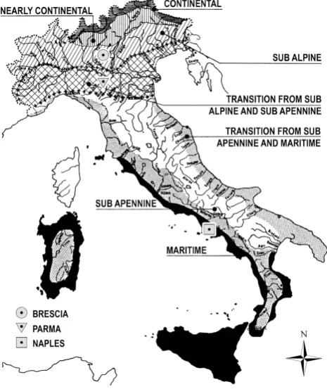
Although they all belong to the Italian peninsula, their cli-mates are quite dissimilar. In the traditional classification proposed by Bandini (1931), illustrated in Fig. 1, the typical Italian rainfall regimes vary from the continental one (with a summer maximum and a winter minimum) to the maritime one (a winter maximum and a summer minimum) and the majority of the territory exhibits an intermediate pluviome-try between these two opposites.

The Brescia series is associated with the sub Alpine cli-mate, which interests the northern portion of the Po Valley and the foothill areas of the tri-Veneto region. Parma lays in-stead in a transition region between the sub-coastal Alpine to sub Apennine climates, that distinguishes the southern part of the Po river catchment and the coastal area of the tri-Veneto. These intermediate regimes are featured by two maximums and two minimums and the range between the extremes is moderate, since it does not exceed 100 % of the monthly an-nual mean.

In the first case, the principal maximum usually occurs in autumn and the secondary one in spring, while the main dry season is in winter; the second case is characterized by a main maximum in autumn and two equal size minimums in summer and in winter. On the contrary, the Naples series originates from the maritime regime, which features Sicily, Sardinia and a large part of the Ionic and Tyrrhenian coasts of southern Italy. Under this boundary regime a single win-ter maximum and a summer minimum occur; hence, the

Fig. 1. Italian precipitation regimes and raingauge locations

(re-drawn from Moisello, 1985).

maximum range is sensibly greater than those typical of the intermediate climates and it can reach up to 200 % of the monthly annual mean (Moisello, 1985).

2.2 Problem formalization

In the copula framework the dependence analysis must rely on uniform random vectors (Joe, 1997), that are gathered from the original ones by means of the Probability Integral Transformation (PIT). In the set of equations written below, the quantities required for this study are defined:

  

x = PV(v)

y = PT(t )

z =PA(a)

with x,y,z∈_I=[0,1], (1)

beingPV,PT andPA the cumulative distribution functions (cdfs) of the original variablesv,t anda, corresponding to thex,yandzdimensionless ones.

Two main advantages arise by employing such transforma-tions: (i) it is easy to prove that they have the same distribu-tion and that this distribudistribu-tion is uniform, (ii) their populadistribu-tion is bounded inside the unitary interval I= [0, 1]. The joint distribution of the original random variables is linked to the copula function by the fundamental Sklar (1959) theorem. In our trivariate case, ifPV T Ais the joint probability function of the rainfall event variables having marginsPV,PT andPA, it allows to state the equality

PV T A = CXY Z[PV(v), PT(t ), PA(a)]. (2)

The function CXY Z: I3→Iis the copula that, in practice, constitutes the joint probability function of the uniform ran-dom variables and defines the dependence structure. The Sklar theorem ensures that such a function exists and, if the marginals are continuous, it is unique. The inference prob-lem of the joint probability functionPV T Afrom the samples derived by the discretization procedure can therefore be sep-arated in the assessment of the copulaCXY Zand of the three univariate distributionsPV,PT andPA.

2.3 Pseudo-observation evaluation

When sample data are considered, the cdfs in Eq. (1) must be approximated. To do this, the plotting positionsFV,FT andFA may be exploited. Herein, in accordance with the standard Weibull formulation, they were expressed as a func-tion of the ranks R(.), associated with the random vector

{ ˆvi,tˆi,aˆi}of dimensionn, as written in Eq. (3) wherexˆi, ˆ

yi andzˆi are usually called pseudo-observations.

       ˆ

xi = FV =

R(vˆi) n+1

ˆ

yi = FT = R(ti)ˆ n+1

ˆ

zi = FA = R(

ˆ ai) n+1

with i = 1, ..., n (3)

A proper estimate of such quantities is essential in the cop-ula framework, even if the sample is affected by ties that could make the rank assignment uncertain. When the pre-cipitation process is considered, the occurrence of a repeated value essentially arises from the discrete nature of the time series, from which the event variables are extracted. Indeed,

it involves both the volume and the duration, because the hyetographs are recorded by using a constant time interval, as a multiple of the minimum depth detectable by the rain-gauge.

As a consequence, if a preliminary data processing is not introduced, the sample contains a large number of minor events distinguished by the lower resolution values both for the volume and the duration (Vandenberghe et al., 2010). On the other hand, the initial discretization required by the analytical-probabilistic approach provides a positive effect on the ties, thanks to its aggregation and filter effects. Fol-lowing this procedure, the single variables, especially the wet weather duration, may still present several repeated values. Nevertheless, the occurrence of a rainfall having contempo-raneously the same characteristics, which is the real concern in the copula assessment perspective, is very rare.

The performed statistical analyses actually revealed that the suppression of the ties does not lead to an appreciable change in the measure of the dependence strength. The ranks in Eq. (3) were calculated by applying the most common for-mulation accounting for all the repeated values, as indicated for the volume in the expression:

R (vi) = n

X

j=1

1 vj ≤ vi

with i =1, ..., n; (4)

in which the 1(.) denotes the indicator function; the adapta-tions for the other variables are obvious.

3 Association measure analysis

The measures of the association degree which relate the uni-form variables combined in pairs, { ˆxi, yˆi}, { ˆyi, zˆi}, and { ˆxi,zˆi}constitute the first step in the assessment of the over-all dependence structure. The use of rank correlation coef-ficients is very convenient inside the copula framework, be-cause of their scale invariant property and non parametric na-ture. Furthermore, a more practical advantage is the possibil-ity to easily relate them to the parameters of the most com-mon copula functions since, unlike the usual Pearson linear correlation measure, they are exclusively a function of the dependence structure.

They represent necessary conditions to determine whether a pair of random variables is independent or not, as well as the traditional Pearson correlation coefficient does, so that they can significantly address the association function selec-tion. In fact, close to zero values suggest the adoption of the independence copula, while some copula families only suit samples which reveal a positive association.

The rank correlation coefficients herein exploited are those defined by Kendall and Spearman. The Kendall coefficientτk

the pairs belonging to a bivariate random vector. The sample versionτˆkof the Kendall coefficient is written in the quotient

ˆ τk =

c−d

c+d; (5)

wherecis the number of concordant data pairs, while d is the number of the discordant ones.

The Spearman coefficientρs (Kruskal, 1958) also relies

on the concordance concept, but its population version has a more complex interpretation. From the copula point of view, it can be regarded as a scalar measure of the average dis-tance between the underlying copula, that rules the random process, and the independence one. Considering for example the bivariate random vector{ ˆxi, yiˆ}, the estimateρˆs of the

Spearman coefficient is given by the relationship

ˆ

ρs = 1 −

6Pn

i=1[R (xi) −R (yi)]2

n3 _−n . (6)

As a result of the scale invariant property of these association measures, the computation does not change if the natural data or the pseudo-observations are employed in the estimators of Eqs. (5) and (6), because the PIT is based on a strictly increasing function.

The sensitivity of the rank correlation measures with re-spect to the independent event separation criteria was as-sessed by varying the two discretization thresholds within quite extended intervals, which were set in consideration of the potential hydrological applications. Hence, the minimum and the maximum IETD values were set in 3 h, correspond-ing to the time of concentration of a medium urban catch-ment, and in 96 h, that could be representative of complex drainage networks equipped with significant storage capaci-ties (Balistrocchi et al., 2009). The IA values were instead set between 1 mm and 10 mm, according to the catchment initial abstractions that could be reasonably assumed in urban and natural catchments, respectively.

Usually, test statistics are employed in order to verify if the rank correlation coefficients are significantly different from zero (see for example Stuart and Ord, 1991). In this case, they yielded results largely consistent with those obtained by the goodness-of-fit tests which are discussed afterwards. Given their greater significance, reporting the achievements of the latter tools was preferred.

3.1 Rainfall volume and wet weather duration pair

When the rainfall volume and the wet weather duration are coupled, the Kendall measure exhibits substantially similar trends in the three locations, as the graphs in the upper part of Fig. 2 demonstrate. The coefficient always assumes posi-tive values from 0.25 to 0.55, outlining a moderately strong concordance between the two variables. Although this range is relatively narrow, they tend to slightly increase with the minimum interevent time but to decrease with the volume threshold. In fact, the weaker association occurs when the

minimum IETD and the maximum IA are set, while the greater one corresponds to the opposite situation.

The first behaviour can be understood by considering the aggregation effect of an increasing IETD on the hyetographs: the longer the minimum interevent time, the greater the wet weather durations and the rainfall depths which characterize the isolated storms are. In addition, the number of indepen-dent events decreases. As a result, the pseudo-observation variability is diminished leading to a more concordant set of pairs. Such a trend is more evident for the lower IETDs, be-cause of the many storm pulses separated by small interevent periods which are present in the series. Further increases in its values determine minor effects and the curves practically tend to assume a constant value.

The second one can only be explained by recognizing that the suppressed low depth events are mainly featured by short durations. Hence, those having high depths but short dura-tions, which form discordant pairs when they are coupled with the major storms, remain in the sample and weaken the overall dependence strength.

The correlation analysis performed by way of the Spear-man concordance measure, whose trends are drawn in the same graphs of Fig. 2, delineates analogous outcomes. The curves of theρs coefficient are shifted upward with respect

to the Kendall ones and the values are enclosed in the in-terval 0.35 and 0.65. Thus, in every climate the pseudo-observations seem to outline very similar dependence struc-tures that are quite different from those due to a couple of independent variables.

These results match the well known empirical evidence, since they confirm the existence of a non negligible statistical association relating the total volume and the duration of an individual storm, according to which the larger precipitation volumes are tendentially generated by the longer wet weather durations. Moreover, its strength demonstrates to be largely independent of the raingauge location. Therefore, the precip-itation regime does not seem to represent a constituent factor in the assessment of this kind of dependence structure, unlike the discretization parameters whose selection determines an appreciable variation in the rank correlation estimate. 3.2 Wet weather duration and interevent period pair

Fig. 2. Trends of the rank correlation coefficients according to the discretization thresholds.

weakness of the relationship can be explained by considering that this occurrence is only characteristic of certain periods, as the summer, when usually very long dry weather periods are interrupted by intense short storms.

In all three climates, theρs behaviour leads to analogous

evaluations, because its curves are overlapped with theτk

ones and substantially follow their trend. Despite the pe-culiarity of the Naples precipitation, the analysis evidences on the whole a random process due to the coupling of two independent variables, in which the absence of a detectable variability with respect to IETD and IA allows to state that their choice is largely trivial.

3.3 Rainfall volume and interevent period pair

When the rainfall volume and the interevent period are joined in pairs, insignificant association degrees are found for all of the series. The curves of the Kendall and Spearman

coefficients, that are drawn in the lower part of Fig. 2, re-veal close to zero values for the majority of the discretization parameter combinations. Only when very high IETD and IA values are set, a small discordant association can be noticed in the Parma and in the Naples series. Such a finding does not seem to be relevant and can be determined by a decrease in the sample size that generates fictitious association strength enhancements.

4 Dependence structure assessment

conditions therefore requires the use of a function able to suit this very asymmetric dependence structure.

One of the most helpful advantages of the copula approach is actually the availability of a number of parametric copula families, whose members can be defined in any multivari-ate case. The majority of models that have found practical application is however fully defined by only one parameter, which is univocally determined by the association degree. In our situation the overall concordance is expected to be low when the three random variables are joined together. Thus, a one-parameter trivariate copula would be close to the in-dependence one and the observed concordance between the event volume and the wet weather duration would not be cor-rectly modelled. Besides, in a multivariate framework hav-ing a dimension greater than two, the concordance estimate is controversial because its definition is ambiguous and com-plex (Salvadori et al., 2007).

A more convenient way is again given by the pairwise analysis, that can exploit various methods for constructing copulas of higher dimension by mixing together also differ-ent bivariate functions; examples are given in Grimaldi and Serinaldi (2006) and Salvadori and De Michele (2006). This technique appeared to be particularly appealing in this appli-cation and was utilized in the following development: firstly one-parameter bivariate copulas were selected and fitted for the three random vectors{xi,yi},{yi,zi}and{xi,zi}, suc-cessively statistical tests were performed for assessing the goodness-of-fit and finally the trivariate function was con-structed and further tested.

4.1 Copula function fitting

The selection of the most suitable copulas relies on the em-pirical copulasCn, whose general expression is written as follows (Ruymgaart, 1973)

Cn(u) = 1 n

n

X

i=1

1 uˆ1,i ≤ u1;...; ˆup,i ≤ up

; (7)

where u=(u1, ..., up) is a p-dimension random vector belonging to Ip, uˆi=(uˆ1,i, ..., uˆp,i) denotes a pseudo-observation vector, 1(.) is the indicator function andnis the sample dimension.

This function computes the frequency of the pseudo-observations whose components do not exceed those of the

uvector and approximates to the underlying copula, in the same manner in which the sample frequency distribution tends to the marginal cumulative probability function. Be-ing Cn a consistent estimator (Deheuvels, 1979), it repre-sents the most objective tool for assessing the dependence structure and can be efficaciously exploited for dealing with the inference problem.

Herein, the copulas taken into consideration were those belonging to the one-parameter families of the Archimedean class, which includes absolutely continuous functions (a wide discussion of their properties is provided by Nelsen,

2006, 106–156 pp.). The choice is justified by the advan-tages of their closed-form expressions and of their versatility, by which they are able to represent a variety of dependence structures both in terms of form and strength. For these rea-sons, the Archimedean copulas have already found applica-tion in many hydrologic problems.

In this situation, the inference problem is simplified in the estimation of the dependence parameter, denoted byθ, of the unknown copulaCunder the null hypothesis

H0:C ∈ C0; (8)

by which the function is a member of a certain parametric family:

C0 = {Cθ:θ ∈ S} with S ⊆ R; (9) beingSa subset of the real number setR.

The fitting methods can be distinguished as either para-metric or semiparapara-metric, in consideration of whether the hy-potheses concerning the marginal distributions are involved or not. The full likelihood criterion and the inference func-tion for margins (Joe, 1997) are parametric methods that em-ploy the Sklar theorem for developing a maximum likelihood estimator where both the marginal and the copula parameters are included.

In the former, all the parameters are simultaneously es-timated by maximizing the log-likelihood function. In the latter, the procedure is divided in two steps: firstly, only the marginal parameters are estimated, by using traditional con-sistent methods. Secondly, the fitted margins are introduced into the log-likelihood function which is maximized to obtain the copula ones. The inference function for margins requires a smaller computational burden than the full likelihood crite-rion, but usually determines an efficiency loss of the estima-tor. Moreover, neither of them leaves the dependence param-eter estimation apart from the detriment due to wrong margin assumptions. In this case, the methods have been proved to be affected by a severe bias (Kim et al., 2007).

One of the most popular semiparametric methods is based on the pseudo-likelihood estimator, that may be expressed as:

L(θ ) =

n

X

i=1

logcθ uˆi

, (10)

wherecθ indicates the copula density (Genest et al., 1995; Shih and Louis, 1995). TheL(θ )function accounts exclu-sively for the pseudo-observation samples, which substitute the marginal cdfs in the estimator argument.

Thus,L(θ )can be interpreted as a further development of the Joe inference function of margins, in which the marginal probabilities are non-parametrically estimated. In general this estimator is less computationally intensive than the pre-vious ones but is not efficient, except for some particular cases (Genest and Werker, 2002).

data by the method of moments. In fact, both the theo-retical versions of Kendall τk and Spearmanρs can be

ex-pressed in terms of theθ parameter. The fitting procedure hence becomes very simple and consists in inverting such relationships and substituting the concordance measure esti-mates gathered from the pseudo-observations.

In our view, despite their limits, the semiparametric meth-ods represent more appropriate tools than the parametric ones, because they are consistent with the copula approach aim, which consists in maintaining the dependence struc-ture assessment independent of those regarding the marginal distributions. Either of these methods can be applied in our case, thanks to the absolute continuity properties of the Archimedean models, that always ensure the existence of the copula density, and thanks to the need for estimating only one dependence parameter.

Considering the volume-duration pair, the most popular Archimedean copulas were fitted to the various random vec-tors{ ˆxi,yˆi}obtained by varying the IETD and the IA thresh-olds and they were visually compared to the corresponding empirical copulas. In the bivariate framework, this may be carried out by drawing the level curves of the two copu-las providing a rough, but effective, evaluation of the global goodness-of-fit.

Among the examined families, the Frank copula (Frank, 1979) and, in particular, the Gumbel-Hougaard copula (Gumbel, 1960; Hougaard, 1986) gave the best adaptations. The bivariate member of this last family was therefore se-lected for modelling the (x, y) distribution by defining the CXY expression as:

CXY(x, y) = expn−(−lnx)θ + (−lny)θ1θ

o

(11)

with x, y ∈ _I.

In this copula the parameterθmust be greater than or equal to one and is univocally determined by the Kendall coefficient τkthrough the relationship:

τk =

θ −1

θ with θ ≥ 1. (12)

The Gumbel-Hougaard family is comprehensive of the inde-pendence copula, which is obtained whenτk is zero andθ

is equal to one, but is able to suit only positively associated data: the stronger the concordance, the higher theθvalue is. The contour plots reveal that the superiority of the Gumbel-Hougaard model with respect to the Frank one is due to its better performance in the upper-right corner of the unitary squareI2, where the larger and more severe occur-rences are located. Indeed, its upper tail behaviour is char-acterized by an asymptotic dependence, lacking in the Frank model, that can be measured by the coefficient:

λu = 2 −21/θ. (13)

The copula density concentrates both in the upper-right cor-ner and in the lower-left one when the association degree in-creases, but only in the former the events appreciably align with the diagonal. This means that such event variables are featured by a deeper association in the extreme storms than in the common rainfalls, which emphasizes the tendency to generate joined values.

When the two calibration criteria were applied, the dif-ferences between the estimations of the dependence param-eter amounted to a few percentage points and no significant detriment or enhancement of the global fit arose by using the method of moment rather than the maximum likelihood criterion. Bearing in mind that the goodness-of-fit tests in-volve a very large number of estimations, the method of mo-ments was preferred to the maximum likelihood estimator in order to limit the computation burden. The estimation of the dependence parameter_θˆ_{was performed by inverting the}

Eq. (12) and substituting the sample versionτˆkof the Kendall

coefficient (Eq. 5).

ˆ

θ = 1

1 − ˆτk

(14) Its behaviour with respect to the discretization thresholds obviously agrees with the one previously discussed for the Kendall coefficient, except for the variability interval. If the same ranges are assumed for the IETD and IA values,θˆis bounded between 1.60 and 2.30; some estimated values are listed in Table 2 for the three series.

As a visual demonstration of the satisfactory goodness-of-fit achievable by using the Gumbel-Hougaard family, the level curves of the theoretical copulas are plotted in Fig. 3 against those of the empirical versions. The samples were derived from the continuous time series by assuming a IETD of 12 h and an IA of 2 mm.

Finally, the independence bivariate copula52was adopted

for the pairs of the interevent period. The bivariate functions CY Z(Eq. 15) andCXZ(Eq. 16) can be defined when the ran-dom variablezis joined to the wet weather durationy and to the rainfall event volume x, respectively. This is a fun-damental copula simply given by the product of the random variables and does not require any calibration.

CY Z(y, z) = 52(y, z) = y z with y, z ∈ I (15)

CXZ(x, z) = 52(x, z) = x z with x, z ∈ I (16)

The suitability of such copulas can be verified by observ-ing the correspondobserv-ing contour plots in Fig. 3, drawn for the samples extracted by using the last mentioned discretization thresholds, where the functions in Eqs. (15) and (16) are compared to their empirical counterparts.

4.2 Copula goodness-of-fit tests

Table 2. Estimations of the dependence parameter_θˆ_{for the precipitation series of Brescia, Parma [.], and Naples (.).}

IETD IA (mm)

(h) 1 4 7 10

3 1.61 [1.94] (1.97) 1.42 [1.57] (1.64) 1.42 [1.46] (1.57) 1.33 [1.44] (1.48) 6 1.75 [1.90] (2.02) 1.50 [1.62] (1.73) 1.45 [1.43] (1.63) 1.39 [1.37] (1.54) 12 1.78 [1.88] (2.14) 1.55 [1.63] (1.86) 1.49 [1.47] (1.68) 1.44 [1.41] (1.60) 24 1.87 [1.88] (2.13) 1.69 [1.72] (1.96) 1.62 [1.56] (1.83) 1.54 [1.47] (1.77) 48 1.92 [2.02] (2.20) 1.77 [1.79] (1.90) 1.68 [1.60] (1.78) 1.63 [1.66] (1.74) 96 2.19 [1.94] (2.29) 2.02 [1.80] (1.93) 1.95 [1.66] (1.89) 1.97 [1.68] (1.90)

Fig. 3. Contour lines of fitted copula functions and empirical copulas for samples extracted by using IETD = 12 h and IA = 4 mm.

a quantitative estimation of the goodness-of-fit by test statis-tic was found to be needed to ensure the model reliability. The test is formally stated with regard to the null hypothesis H0 (Eq. 8), under which the copulas were fitted. The

ob-jective is to verify whether the underlying unknown copula

belongs to the chosen parametric family or such an assump-tion has to be rejected.

are classified by the Authors in three main categories (i) those that can be utilized only for a specific copula family (Shih, 1998; Malevergne and Sornette, 2003), (ii) those that have a general applicability but involve important subjective choices for their implementation, such as a parameter (Wang and Wells, 2000), a smoothing factor (Scaillet, 2007) or a data categorization (Junker and May, 2005), (iii) those that do not have any of the previous constraints and for this reason are called blanket tests. The convenience of adopting the last kind of test is clear and was highlighted by the Authors them-selves.

Furthermore, in the same paper, they analyzed the perfor-mances of some blanket procedures by way of large scale Montecarlo simulations, obtaining a general confirmation of their validity. One of the most powerful tests is based on the empirical copula process_Cndefined as:

Cn = √

n Cn −C_θˆ

, (17)

which evaluates the distance between the empirical copula Cnand the estimateC_θˆof the underlying copulaCunder the null hypothesisH0.

A suitable test statisticSn can be constructed by using a rank-based version of the Cramer-Von Mises criterion, as written in the integral:

Sn =

Z

[0,1]p

Cn(u)2dCn(u) with u ∈ Ip, (18)

whose integration variable u is a generic uniform random vector having p dimension. When the Sn values are low, the fitted model and the pseudo-observation distribution are close, on the contrary, they disagree considerably. In the first condition the null hypothesisH0cannot be rejected, while in

the other it can.

Dealing with the pseudo-observationsuˆi, the statisticSn may be approximated by the sum:

Sn =

n

X

i=1

Cn uˆi −C_θˆ uˆi2. (19)

As previously argued by Fermanian (2005) and successively demonstrated by Genest and R´emilland (2008), the statis-tic Sn is able to yield an approximate p-value if it is im-plemented inside an appropriate parametric bootstrap proce-dure. According to the achievements previously discussed, in our case the procedure was implemented as follows, for each of the three pairs of random variables:

– For a given combination of the parameter IETD and IA, nbivariate vectors of pseudo-observations are derived by using the discretization procedure described in chap-ter 2, beingnthe total number of independent storms. – The sample Kendall coefficient τˆk and the empirical

copulaCn are computed with respect to the observed data by their expressions in Eqs. (5) and (7).

– The dependence parameter_θˆ_{is estimated by the method}

of moments, assessing the underlying copulaC_θˆ. – The Cramer-Von Mises statisticSnis directly calculated

by Eq. (19), in which the analytical formulation of the Archimedean models is utilized.

– For a large integerN, the next sub-steps are repeated for everym= 1, ...,N:

– A sample of pseudo-observations ofndimension is generated by simulating the estimation of the un-derlying copulaC_θˆ.

– The sample Kendall coefficientτˆk,mand the empiri-cal copulaCn,mof the simulated data are computed by using their expressions in Eqs. (5) and (7). – The dependence parameter_θmˆ _{is estimated by the}

method of moments, assessing the theoretical cop-ulaC_θˆ

m.

– The Cramer-Von Mises statisticSn,m of the simu-lated sample is calcusimu-lated by the same expression of Eq. (19), in whichCn,mandC_θmˆ are substituted toCnandC_θˆ, respectively.

– An approximatep-value is finally provided by the sum: 1

N N

X

m=1

1 Sn,m > Sn. (20)

The tests were conducted varying the discretization parame-ters within the same IETD and IA ranges previously used for the association measure analysis. Firstly, the real existence of an association degree was verified by assuming that all the three bivariate distributions correspond to the independent 2-copula (Eq. 21). When this assumption is tested, the proce-dure simplifies, because the steps concerning the estimation of the dependence parameter do not apply.

H0:C = 52 (21)

Thep-values listed in Tables 3, 4 and 5 were obtained for the three couples by assumingN greater than 2500. On the whole, the independence assumption must be rejected for the event volume and the wet weather duration pair, because null or close to zerop-values are assessed, while for the other two variable joints it cannot be rejected with significance levels considerably greater than the usual values of the 5:10 %. In addition, no particular trends with regard to the IETD and IA settings or differences among the climates are detected.

Hence, only for the first couple the null hypothesis (Eq. 22), by which the dependence structure can be modeled by the Gumbel-Hougaard 2-copula, was examined. Additional goodness-of-fit tests supplied the estimations that are listed in Table 6.

H0:CXY ∈

exp

−(−lnx)θ + (−lny)θ

1 θ

:θ ∈ [1,∞[

Table 3.p-values (%) obtained when testing the independence between the event volume and the wet weather duration for the rainfall series of Brescia, Parma [.], and Naples (.).

IETD IA (mm)

(h) 1 4 7 10

3 0.0 [0.0] (0.0) 0.0 [0.0] (0.0) 0.0 [0.0] (0.0) 0.0 [0.4] (0.0) 6 0.0 [0.0] (0.0) 0.0 [0.0] (0.0) 0.0 [0.0] (0.0) 0.0 [1.2] (0.0) 12 0.0 [0.0] (0.0) 0.0 [0.0] (0.0) 0.0 [0.2] (0.0) 0.0 [0.6] (0.0) 24 0.0 [0.0] (0.0) 0.0 [0.0] (0.0) 0.0 [0.0] (0.0) 0.0 [0.3] (0.0) 48 0.0 [0.0] (0.0) 0.0 [0.0] (0.0) 0.0 [0.0] (0.0) 0.0 [0.0] (0.0) 96 0.0 [0.0] (0.0) 0.0 [0.0] (0.0) 0.0 [0.1] (0.0) 0.0 [0.3] (0.0)

Table 4.p-values (%) obtained when testing the independence between the wet weather duration and the interevent period for the rainfall series of Brescia, Parma [.], and Naples (.).

IETD IA (mm)

(h) 1 4 7 10

3 81.1 [78.6] (84.0) 42.2 [97.8] (82.8) 47.6 [100.0] (98.5) 65.9 [100.0] (96.0) 6 85.0 [96.9] (91.6) 79.0 [97.2] (78.2) 87.7 [100.0] (66.5) 73.8 [100.0] (59.0) 12 66.2 [100.0] (100.0) 79.7 [100.0] (89.8) 87.6 [100.0] (86.7) 85.8 [100.0] (54.1) 24 99.9 [100.0] (94.3) 100.0 [99.0] (92.0) 100.0 [94.0] (99.7) 100.0 [99.8] (97.8) 48 99.2 [96.8] (99.8) 99.9 [98.7] (94.2) 96.6 [99.8] (96.4) 77.6 [100.0] (100.0) 96 100.0 [100.0] (100.0) 99.9 [100.0] (100.0) 99.8 [100.0] (100.0) 100.0 [100.0] (98.0)

Thep-values mainly range between 40 % and 100 %, demon-strating that the selected family is able to suit the empirical data, ensuring very high significance levels for all the IETD and IA choices and the precipitation regimes. Nevertheless, the goodness-of-fit shows a moderate tendency to improve according to the increments of both the discretization pa-rameters. The Frank model was tested as well, but in nearly every case poorer adaptations (50:60 %) were evidenced by p-values lower than the Gumbel-Hougaard ones. The only exception was noticed in the Brescia rainfall series for the minor thresholds, for which thep-values of the two models are however comparable.

The p-values exactly equal to the unity could certainty seem anomalous. The occurrence may be explained by the limited number N of repeated simulations that were per-formed, which was not set substantially larger than the sam-ple dimensionnas recommended by Genest et al. (2009) for limiting the estimation variance. This choice was due to the need to balance the assessment accuracy and the heavy com-putational demand of the procedure, since the sample sizes can greatly exceed two thousand when the lower values are utilized for the discretization thresholds. An iteration num-ber of 2500 has been considered by the same Authors as an acceptable compromise, that still allows to meet the main ob-jective of the test, even though a certain loss of the estimator efficiency has to be accounted for. Indeed, in our application,

the assessedp-values do not demonstrate any relevant vari-ations when the procedure is carried out by repeating over 2000 simulations.

Thus, it can be concluded that the goodness-of-fit tests based on the Cramer-Von Mises statisticSn definitely con-firm the broad framework that has been delineated by the as-sociation measure analysis and by the graphical fits, since the assumed bivariate models cannot be rejected for the standard significance levels commonly adopted in the statistical tests. 4.3 Mixing method

Among quite a large set of strategies for constructing mul-tivariate copulas, the conditional approach that was investi-gated by Chakak and Koehler (1995) seemed to be extremely convenient. In fact, it is possible to demonstrate that the trivariate copulaCXY Zmust satisfy the equality

CXY Z(x, y, z) = CXY

_C

XZ(x, z)

z ,

CY Z(y, z) z

z (23)

which mixes together the lower order copulas.

Table 5.p-values (%) obtained when testing the independence between the event volume and the interevent dry period for the rainfall series of Brescia, Parma [.], and Naples (.).

IETD IA (mm)

(h) 1 4 7 10

3 91.0 [100.0] (100.0) 100.0 [92.8] (94.2) 100.0 [90.4] (84.3) 99.8 [100.0] (100.0) 6 98.0 [100.0] (100.0) 99.8 [88.8] (100.0) 100.0 [89.7] (99.5) 100.0 [99.8] (99.8) 12 75.2 [100.0] (99.9) 100.0 [100.0] (99.3) 100.0 [99.8] (99.7) 98.4 [100.0] (99.4) 24 94.8 [99.6] (100.0) 99.9 [99.6] (100.0) 99.5 [99.8] (100.0) 91.0 [100.0] (99.7) 48 100.0 [100.0] (100.0) 100.0 [100.0] (100.0) 100.0 [100.0] (100.0) 100.0 [100.0] (100.0) 96 100.0 [100.0] (99.4) 100.0 [99.4] (97.4) 100.0 [98.1] (99.8) 100.0 [99.5] (74.7)

Table 6.p-values (%) obtained when testing the goodness-of-fit of the Gumbel-Hougaard model to the event volume and the wet weather duration pair for the rainfall series of Brescia, Parma [.], and Naples (.).

IETD IA (mm)

(h) 1 4 7 10

3 39.1 [100.0] (98.7) 77.2 [100.0] (99.8) 90.9 [99.9] (100.0) 100.0 [100.0] (99.8) 6 77.0 [99.7] (99.2) 97.6 [100.0] (100.0) 100.0 [100.0] (99.6) 99.9 [100.0] (98.8) 12 91.9 [100.0] (100.0) 96.8 [100.0] (100.0) 100.0 [100.0] (99.5) 99.9 [100.0] (99.2) 24 99.7 [100.0] (100.0) 99.9 [100.0] (100.0) 100.0 [100.0] (100.0) 100.0 [100.0] (100.0) 48 98.4 [100.0] (100.0) 100.0 [100.0] (100.0) 100.0 [100.0] (100.0) 100.0 [100.0] (100.0) 96 100.0 [100.0] (100.0) 99.0 [100.0] (100.0) 91.7 [100.0] (100.0) 98.3 [100.0] (100.0)

equation of the trivariate copula is easily reduced to the prod-uct of the bivariate copulaCXY and the uniform variablez.

CXY Z(x, y, z) =CXY

₅

2(x, z)

z ,

52(y, z)

z

z (24)

=CXY

x z z ,

y z z

z = CXY(x, y) z

Thus, the joint distribution suiting the natural variability of the individual rainfall event variables may be expressed by the trivariate copula in Eq. (25), whose unique parameterθ is exclusively a function of the positive association between the event volume and the wet weather duration.

CXY Z(x, y, z) = exp

−(−lnx)θ + (−lny)θ 1 θ

z (25)

When goodness-of-fit tests were performed for this trivariate copula function,p-values mainly ranging between 40 % and 100 % were found. Such a result was expected in view of the highp-values obtained in the pair analysis and definitely supports the reliability of the proposed copula function for the three precipitation regimes. The detailedp-value varia-tion with respect to the discretizavaria-tion thresholds is reported in Table 7.

5 Marginal distribution assessment

Several probability models have been suggested for describ-ing the natural variability of the rainfall event characteristics, including the Gamma (Di Toro and Small, 1979; Wood and Hebson, 1986), the Pareto (Salvadori and De Michele, 2006) and the Poisson functions (Wanielista and Yousef, 1992). Nonetheless, the most popular one is certainly the exponen-tial model, that has been extensively employed in a huge number of problems (a detailed list is provided in Salvadori and De Michele, 2007). The reason for such a success mainly lies in its very simple formula, that often allows to analyti-cally integrate the derived probability functions and therefore makes it particularly appealing in the analytical-probabilistic perspective.

Unfortunately, in the Italian precipitation regimes the ex-ponential model does not suit the observed distributions of the rainfall event variables. An appropriate alternative has been identified in the Weibull model, that can be viewed as a more versatile generalization of the exponential one. Hence, the theoretical marginalsPV,PT andPA defined in Eq. (1) have been represented by means of the three cdfs in Eqs. (26), (27) and (28), respectively.

PV(v) =

  

1 −exp

−v−IA ζ

β

for v ≥ IA

0 otherwise

Table 7.p-values (%) obtained when testing the trivariate copula for the rainfall series of Brescia, Parma [.], and Naples (.).

IETD IA (mm)

(h) 1 4 7 10

3 43.3 [98.7] (99.7) 41.3 [99.8] (95.2) 73.0 [99.8] (94.4) 99.5 [99.9] (99.5) 6 75.0 [99.9] (99.7) 70.4 [98.2] (98.2) 96.6 [99.9] (95.8) 80.0 [99.5] (91.9) 12 65.0 [100.1] (92.1) 87.6 [100.0] (98.2) 93.1 [100.0] (99.6) 83.0 [99.7] (82.6) 24 99.0 [99.5] (99.9) 99.8 [96.6] (99.9) 99.4 [79.1] (100.0) 96.8 [99.3] (99.8) 48 97.7 [99.9] (100.1) 99.9 [100.0] (99.4) 99.4 [100.0] (98.5) 98.6 [100.0] (99.9) 96 100.0 [100.0] (96.9) 99.4 [100.0] (99.5) 91.8 [98.0] (99.9) 99.2 [99.2] (67.5)

PT(t ) =

1 − exp− t λ

γ

for t ≥ 0

0 otherwise (27)

PA(a) =

  

1− exp

−

a−IETD

ψ

δ

for a ≥ IETD

0 otherwise

(28)

The exponentsβ,γ andδare dimensionless parameters that rule the shape of the distributions, while the denominatorsζ (mm),λ(h) andψ(h) define the scale of the random process. The IA and the IETD parameters represent the lower limits in Eqs. (26) and (28) and are set in accordance with the min-imum interevent time and the volume threshold employed in the rainfall separation procedure.

In this kind of model the correct assessment of the expo-nent is a key aspect, because very dissimilar shapes of the probability density function (pdf) are possible with respect to its value: (i) when an exponent smaller than one occurs, the pdf monotonically decreases from the lower limit in which a vertical asymptote is present, (ii) when it is exactly equal to one, the pdf owns a finite mode in the lower limit but does not lose the monotonic decreasing behaviour, (iii) when it ex-ceeds the unity the distribution mode is greater than the lower limit and the pdf exhibits a right tail that is progressively less marked if it is further incremented. Hence, the greater the ex-ponent, the more shifted to the right the most probable values are and the more symmetric the distribution is.

5.1 Marginal function fitting

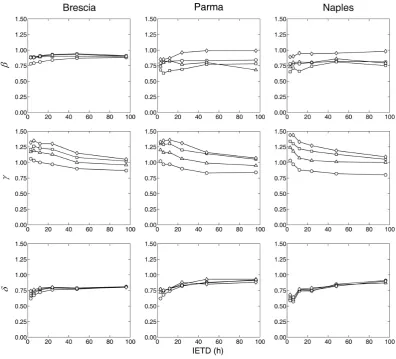
A sensitivity analysis has been carried out referring to the previously investigated IETD and IA ranges. The marginal distributions were fitted to the sample data extracted from the continuous rainfall series by the maximum likelihood crite-rion yielding the graphs plotted in Fig. 4 for the shape pa-rameters and in Fig. 5 for the scale ones: on the whole, it can be argued that the precipitation regime does not significantly affect the estimation of the margin parameters, since almost identical behaviours are evidenced.

The shape parametersβ andδ are always less than the unity, because they lie within the intervals 0.60:0.98 and 0.55:0.90, respectively; on the contrary, the exponentγ of

the storm duration cdf may be greater than one, being es-timated between 0.80:1.35. As mentioned above, the unity represents a fundamental boundary for the shape parameter. Therefore, unlike the other two distributions, the duration pdf may be subject to important changes in shape with reference to the discretization parameter settings.

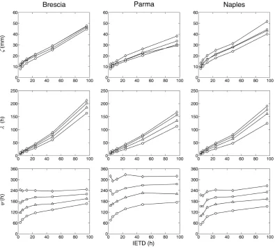
For all the three exponents, greater values are generally es-timated when the volume threshold increases, while different trends are evidenced with respect to the minimum interevent time. In fact, theδexponent increases with the IETD, but the opposite behaviour occurs for theγ exponent and, finally, no clear tendency can be detected for theβ exponent. The scale parametersζ,λandψare instead characterized by a wider variability, by which they increase according to both the discretization thresholds in quite a proportional manner.

The reasons for such outcomes reside in the effects of the discretization thresholds, illustrated in the association anal-ysis context. The scale parameters mainly depend on the mean, whose increments can be immediately justified by the isolation of more extended events separated by longer dry weather periods. The shape parameters are instead essen-tially related to the variance; given the wide scale variability, the dispersion around the mean must be discussed by using the coefficient of variation, which is exclusively a function of the exponent.

The properties of the Weibull probability function are such that the exponent increase is related to a reduction of the co-efficient of variation. In fact, if the volume threshold is incre-mented the frequency of the smallest observations decreases for all three variables, diminishing the overall distribution dispersion. An analogous explanation may be advanced for understanding the effects of the IETD extension on the dry whether period distribution, because the minimum interevent time directly acts on the variable as a threshold.

Fig. 4. Trends of the margin shape parameters according to the discretization thresholds.

the standard deviation, leading to the reduction of the coeffi-cient of variation.

Finally, the lack of a recognizable trend of the rainfall volume dispersion with respect to the IETD appears to be reasonable because this discretization parameter operates re-gardless of this quantity: even storms having completely dif-ferent depths may be joined into a unique event and so the dispersion change is not univocally foreseeable.

The scale parameters deserve a last consideration because, albeit they do not seem to be sensitive to the precipitation regime, they evidence however to be influenced by another climatic aspect such as the annual precipitation amount. Ob-viously, in the wetter climates, greaterζ andλvalues have been estimated, while the dryer ones were found to be fea-tured by largerψ. A demonstration of this assertion can be found in Fig. 5 by observing the curves belonging to the Parma series, whose annual mean depth is the lowest among the presented cases.

5.2 Marginal goodness-of-fit tests

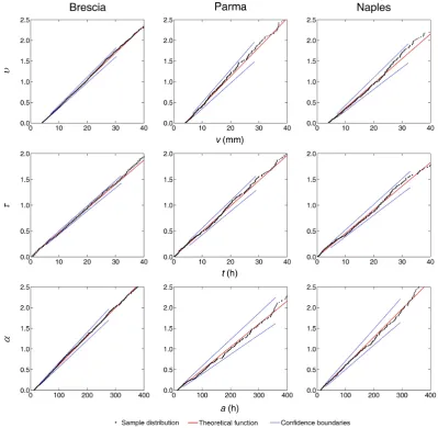
The suitability of the Weibull probabilistic model for repre-senting the natural variability of the rainfall event volumes has already been proved by using the confidence boundary test for the Brescia time series (Bacchi et al., 2008). In this work, the same technique has been adopted for assessing the goodness-of-fit in all the illustrated Italian climates regarding the complete set of random variables. The tests are intended to verify whether the Weibull distributions from Eq. (26) to Eq. (28), fitted by way of the maximum likelihood method, can be rejected or not according to an a priori fixed signif-icance level. They are based on the standard variablesυ,τ andαdefined for the event volume, the wet weather duration and the interevent periods respectively

υ = v −IA

ˆ ζ

;τ = t ˆ λ

;α = a −IETD ˆ

Fig. 5. Trends of the margin scale parameters according to the discretization thresholds.

The corresponding sample versions are easily obtained by inverting the cdfs and substituting the frequenciesF (Eq. 2) to the non exceedance probabilityP:

ˆ

υ =

ln

₁

1 −FV

1_ˆ

β ; ˆτ =

ln

₁

1−FT

_γ1_ˆ

; (30)

ˆ

α =

ln

₁

1 −FA

1_ˆ

δ .

The confidence limits were centered with respect to the the-oretical value and quantified for a significance level of 5 % by using the interval half-width1in Eq. (31), computed as a function of the non exceedance probabilityP and the proba-bility densitypof the standard variable.

1 = ± 1√.96 n

√

P (1 −P )

p (31)

An example of the goodness-of-fit achievable by means of the Weibull probabilistic model is illustrated in the plots of

Fig. 6, in which the confidence boundaries are drawn be-tween the probability interval 0.20:0.80 and the sample data are derived from the continuous record by using the thresh-olds IETD = 12 h and IA = 4 mm. The sample points are fairly aligned with the theoretical line and substantially en-compassed in the confidence region. Analogous results were gathered from all the series by using different sets of IETD and IA. Thus, in general, the hypothesis concerning the as-sumed probabilistic function cannot be rejected.

6 Conclusions

Fig. 6. Margin goodness-of-fit tests for samples extracted by using IETD = 12 h and IA = 4 mm.

time series, which may be operatively defined with regard to the derived hydrological process involved in the application. The copula functions played a fundamental role in the de-velopment of the joint distribution function relating to these variables. The essential advantages consisted in the capa-bility of constructing unconventional functions by exploiting mixing techniques applied to bivariate copulas and in testing the model components separately. The first aspect ensures a considerable enhancement of the model suiting capacity, while the second one is significantly involved in the control of the computational burden.

In general, it must be pointed out that the copula approach provides a rigorous and objective procedure to face the in-ference problem in the multivariate framework and to avoid the heuristic approaches and the arbitrary assumptions that affected the joint distribution assessment in the past. Hence, the extreme convenience of this approach must be strongly

highlighted and its systematic utilization may be definitely advocated.

This provides a reason for the difficulties encountered in the stochastic representation of the dependent hydrological variables. On the contrary, when the interevent dry period is joined to the other variables, the independence hypothe-sis cannot be rejected, confirming the reliability of the tradi-tional assumption.

The ability of the three parameter Weibull function to fit the marginal distributions of all the analysed random vari-ables was also statistically tested. In the proposed formula-tion, the distribution lower limit is a priori fixed with refer-ence to the independent event discretization procedure, while the other two may be estimated by the maximum likelihood criterion. The main appeal of using this alternative model lies in its analytical form, that neither compromises the model versatility required by the sample data nor complicates the parameter assessment.

The analysis took into consideration three time series, which are representative of as many Italian rainfall regimes. Despite the variability of their meteorological characteris-tics, the analysis revealed that, when the thresholds employed for isolating the independent storms change, both the depen-dence structure and the margins show identical behaviours. Moreover, very similar fitting values were estimated for their parameters, except for those expressing the univariate dis-tribution scale which demonstrated to be moderately influ-enced by the total annual rainfall depth. A very satisfactory agreement between theoretical functions and observed data is outlined by the performed statistical tests, for every couple of IETD and IA values that were considered. Thus, a gen-eral reliability of the proposed probabilistic model may be deduced for the Italian climates.

The natural research development could be addressed to the flood frequency analysis, by exploiting deterministic or stochastic routing models, or to the watershed hydrologic balance, considered both in its global terms and in its com-ponents, infiltration and evapotranspiration. Even though the proposed model has quite a simple expression, its implemen-tation in the derivation procedure should reasonably yield pdfs that cannot be analytically integrated. The model ef-fectiveness advance will have to be carefully appraised in consideration of such an inconvenience, since the capabil-ity of the analytical-probabilistic methodology to express the derived probability functions by an analytical expression rep-resents one of the most important advantages that justifies its use.

Finally, another research perspective is offered by the con-cerns involved in the estimation of the return period. In fact, in the multivariate case its evaluation still remains an open question, because a universally accepted definition has not been proposed yet. The main reason lies in the ambiguity of having very different events associated with the same fre-quency of occurrence, which arises from the most immediate generalizations of this concept. The analytical-probabilistic methodology offers a way of facing this problem from the

univariate point of view, because the forcing meteorological variables are directly related to the dependent one.

Acknowledgements. Giuseppe De Martino of the University Federico II and his research group are kindly acknowledged for having provided the Naples precipitation data. The reviewers and Gianfausto Salvadori of the University of Lecce are also acknowledged for their useful suggestions and fruitful discussions. The research was supported by grants from the University of Brescia.

Edited by: A. Montanari

References

Adams, B. J., and Papa, F.: Urban stormwater management plan-ning with analytical probabilistic models, John Wiley & Sons, New York, 2000.

Bacchi, B., Becciu, G., and Kottegoda, N. T.: Bivariate exponential model applied to intensities and durations of extreme rainfall, J. Hydrol., 155(1–2), 225–236, doi:10.1016/0022-1694(94)90166-X, 1994.

Bacchi, B., Balistrocchi, M., and Grossi, G.: Proposal of a semi-probabilistic approach for storage facility design, Urban Water J., 5(3), 195–208, doi:10.1080/15730620801980723, 2008. Balistrocchi, M., Grossi, G., and Bacchi, B.: An analytical

prob-abilistic model of the quality efficiency of a sewer tank, Water Resour. Res., 45, W12420, doi:10.1029/2009WR007822, 2009. Bandini, A.: Tipi pluviometrici dominanti sulle regioni italiane,

Servizio Idrografico Italiano, Roma, Italy, 1931.

Beven, K. J.: Rainfall-runoff modelling: the primer, John Wi-ley & Sons, Bath, UK, 2001.

Bonta, J. V. and Rao, A. R.: Factors affecting the identifica-tion of independent storm events, J. Hydrol., 98(3–4), 275–293, doi:10.1016/0022-1694(88)90018-2, 1988.

Chakak, A. and Koehler, K. J.: A strategy for constructing multi-variate distributions, Commun. Stat. Simulat., 24(3), 537–550, doi:10.1080/03610919508813257, 1995.

Chan, S.-O. and Bras, R. L.: Urban storm water management: dis-tribution of flood volumes, Water Resour. Res., 15(2), 371–382, doi:10.1029/WR015i002p00371, 1979.

Chow, V. T., Maidment, D. R., and Mays, L. W.: Applied hydrology, McGraw-Hill International Edition, New York, NY, USA, 1988. C´ordova, J. R. and Rodr´ıguez-Iturbe, I.: On the probabilistic struc-ture of storm surface runoff, Water Resour. Res., 21(5), 755–763, doi:10.1029/WR021i005p00755, 1985.

Cox, D. R. and Isham, V.: Point processes, Chapman and Hall Ltd., London, UK, 1980.

Deheuvels, P.: Empirical dependence function and properties: non-parametric test of independence, Bulletin de la classe des sci-ences Academie Royale de Belgique, 65(6), 274–292, 1979. Di Toro, D. M. and Small, M. J.: Stormwater interception and

stor-age, J. Environ. Eng.-ASCE, 105(1), 43–54, 1979.

D´ıaz-Granados, M. A., Valdes, J. B., and Bras, R. L.: A physically based flood frequency distribution, Water Resour. Res., 20(7), 995–1002, doi:10.1029/WR020i007p00995, 1984.

Eagleson, S. P.: Dynamics of flood frequency, Water Resour. Res., 8(4), 878–898, doi:10.1029/WR008i004p00878, 1972.

Eagleson, S. P.: Climate, soil, and vegetation 2. The dis-tribution of annual precipitation derived from observed storm sequences, Water Resour. Res., 14(5), 713–721, doi:10.1029/WR014i005p00713, 1978a.

Eagleson, S. P.: Climate, soil, and vegetation 5. A derived distribu-tion of storm surface runoff, Water Resour. Res., 14(5), 741–748, doi:10.1029/WR014i005p00741, 1978b.

Eagleson, S. P.: Climate, soil and vegetation 7. A derived distribu-tion of annual water yield, Water Resour. Res., 14(5), 765–776, doi:10.1029/WR014i005p00765, 1978c.

Fermanian, J.-D.: Goodness-of-fit tests for copulas, J. Multivar. Anal., 95(1), 119–152, doi:10.1016/j.jmva.2004.07.004, 2005. Foufoula-Georgiou, E. and Guttorp, P.: Assessment of a class of

Neyman-Scott models for temporal rainfall, J. Geophys. Res., 92(D8), 9679–9682, doi:10.1029/JD092iD08p09679, 1987. Frank, M. J.: On the simultaneous associativity of F (x,y)

and x+y−F (x,y), Aequationes Math., 19(1), 194–226, doi:10.1007/BF02189866, 1979.

Genest, C. and R´emilland, B.: Validity of the parametric bootstrap for goodness-of-fit testing in semiparametric models, Annales de l’Institut Henri Poincar´e: Probabilit´es et Statistiques, 44 (6), 1096–1127, 2008.

Genest, C. and Werker, B. J. M.: Conditions for the asymptotic semiparametric efficiency of an omnibus estimator of depen-dence parameters in copula models, in: Distribution with Given Marginals and Statistical Modelling, Kluwer, Dordrecht, The Nederlands, 103–112, 2002.

Genest, C., Ghoudi, K., and Rivest, L.-P.: A semiparamet-ric estimation procedure of dependence parameters in multi-variate families of distributions, Biometrika, 82(3), 543–552, doi:10.1093/biomet/82.3.543, 1995.

Genest, C., R´emilland, B., and Beaudoin, D.: Goodness-of-fit tests for copulas: a review and a power study, Insur. Math. Econ., 44(2), 199–213, doi:10.1016/j.insmatheco.2007.10.005, 2009. Goel, N. K., Kurothe, R. S., Mathur, B. S., and Vogel, R. M.: A

de-rived flood frequency distribution for correlated rainfall intensity and duration, J. Hydrol., 228(1–2), 56–67, doi:10.1016/S0022-1694(00)00145-1, 2000.

Grimaldi, S. and Serinaldi, F.: Asymmetric copula in multivariate flood frequency analysis, Adv. Water Resour., 29(8), 1115–1167, doi:10.1016/j.advwatres.2005.09.005, 2006.

Gumbel, E. J.: Distributions des valeurs extr´emes en plusieurs di-mensions, Publ. Inst. Statist. Univ. Paris 9, 171–173, 1960. Guo, Y. and Adams, B. J.: Hydrologic analysis of urban

catchments with event-based probabilistic models 2. Peak discharge rate, Water Resour. Res., 34(12), 3433–3443, doi:10.1029/98WR02448, 1998.

Guo, Y. and Adams, B. J.: An analytical probabilistic approach to sizing flood control detention facilities, Water Resour. Res., 35(8), 2457–2468, doi:10.1029/1999WR900125, 1999. Hougaard, P.: A class of multivariate failure time distributions,

Biometrika, 73(3), 671–678, doi:10.1093/biomet/73.3.671, 1986.

Joe, H.: Multivariate models and dependence concepts, Chapman and Hall, London, 1997.

Junker, M. and May, A.: Measurement of aggregate risk with copulas, Economet. J., 8(3), 428–454, doi:10.1111/j.1368-423X.2005.00173.x, 2005.

Kendall, M. G.: A new measure of the rank correlation, Biometrika, 30(1–2), 81–93, doi:10.1093/biomet/30.1-2.81, 1938.

Kim, G., Silvapulle, M. J., and Silvapulle, P.: Compari-son of semiparametric and parametric methods for estimat-ing copulas, Comput. Stat. Data. An., 51(6), 2836–2850, doi:10.1016/j.csda.2006.10.009, 2007.

Kruskal, W. H.: Ordinal Measures of Association, J. Am. Stat. As-soc., 53(284), 814–861, doi:10.2307/2281954, 1958.

Kurothe, R. S., Goel, N. K., and Mathur, B. S.: Derived flood frequency distribution for negatively correlated rainfall in-tensity and duration, Water Resour. Res., 33(9), 2103–2107, doi:10.1029/97WR00812, 1997.

Li, J. Y. and Adams, B. J.: Probabilistic models for analysis of ur-ban runoff control systems, J. Environ. Eng., 126(3), 217–224, doi:10.1061/(ASCE)0733-9372(2000)126:3(217), 2000. Malevergne, Y. and Sornette, D.: Testing the Gaussian copula

hy-pothesis for financial assets dependences, Quant. Financ., 3(4), 231–250, doi:10.1088/1469-7688/3/4/301, 2003.

Moisello, U.: Grandezze e fenomeni idrologici, La Goliardica Pavese, 1985.

Nelsen, R. B.: An introduction to copulas, 2 edition, Springer, New York, 2006.

Restrepo-Posada, P. J. and Eagleson, P. S.: Identification of independent rainstorms, J. Hydrol., 55(1–4), 303–319, doi:10.1016/0022-1694(82)90136-6, 1982.

Ruymgaart, F. H.: Asymptotic theory for rank tests for indepen-dence, MC Tract 43, Amsterdam, Mathematisch Instituut, 1973. Salvadori, G. and De Michele, C.: Statistical characterization of temporal structure of storms, Adv. Water Resour., 29(6), 827– 842, doi:10.1016/j.advwatres.2005.07.013, 2006.

Salvadori, G. and De Michele, C.: On the use of copulas in hydrol-ogy: theory and practice, J. Hydrol. Eng.-ASCE, 12(4), 369–380, doi:10.1061/(ASCE)1084-0699(2007)12:4(369), 2007. Salvadori, G., De Michele, C., Kottegoda, N. T., and Rosso, R.:

Extremes in nature: an approach using copulas, Springer, Dor-drecht, The Nederlands, 2007.

Scaillet, O.: Kernel-based goodness-of-fit tests for copulas with fixed smoothing parameters, J. Multivar. Anal., 98(3), 533–543, doi:10.1016/j.jmva.2006.05.006, 2007.

Seto, M. Y. K.: Comparison of alternative derived probability distri-bution models for urban stormwater management, M.A.Sc. the-sis, Department of Civil Engineering, University of Toronto, Toronto, Ontario, 1984.

Shih, J. H.: A goodness-of-fit test for association in a bi-variate survival model, Biometrika, 85(1), 189–200, doi:10.1093/biomet/85.1.189, 1998.

Shih, J. H. and Louis, T. A.: Inferences on the association parameter in copula models for bivariate survival data, Biometrics, 51(4), 1384–1399, 1995.

Singh, K. and Singh, V. P.: Derivation of bivariate probability den-sity functions with exponential marginals, Stoch. Hydrol. Hy-draul., 5(1), 55–68, doi:10.1007/BF01544178, 1991.

Stuart, A. and Ord, J. K.: Kendall’s advanced theory of statistics, 5th edition, Vol. 2, Edward Arnold, London, UK, 1991. Vandenberghe, S., Verhoest, N. E. C., and De Baets, B.: Fitting

bi-variate copulas to the dependence structure between storm char-acteristics: a detailed analysis based on 105 year 10 min rainfall, Water Resour. Res., 46, W01512, doi:10.1029/2009WR007857, 2010.

Wang, W. J. and Wells, M. T.: Model selection and semiparamet-ric inference for bivariate failure-time data, J. Am. Stat. Assoc., 95(449), 62–72, 2000.

Wanielista, M. P. and Yousef, Y. A.: Stormwater management, John Wiley & Sons, New York, 1992.

Waymire, E., Gupta, V. K., and Rodriguez-Iturbe, I.: A spectral the-ory of rainfall intensity at the meso-βscale, Water Resour. Res., 20(10), 1453–1465, doi:10.1029/WR020i010p01453, 1984. Wood, E. F. and Hebson, C. S.: On hydrologic similarity 1.