www.hydrol-earth-syst-sci.net/16/761/2012/ doi:10.5194/hess-16-761-2012
© Author(s) 2012. CC Attribution 3.0 License.
Earth System
Sciences
Characterization of deep aquifer dynamics using principal
component analysis of sequential multilevel data
D. Kurtzman1, L. Netzer2, N. Weisbrod2, A. Nasser1, E. R. Graber1, and D. Ronen2,3
1Institute of Soil, Water and Environmental Sciences, The Volcani Center, Agricultural Research Organization,
P.O. Box 6, Bet Dagan 50250, Israel
2Department of Hydrology & Microbiology, Zuckerberg Institute for Water Research, Blaustein Institutes for
Desert Research, Ben Gurion University of the Negev, Sde Boker Campus, Negev 84990, Israel
3Hydrological Service and Water Quality Division, Israel Water Authority, P.O. Box 20365, Tel Aviv 61203, Israel Correspondence to: D. Kurtzman ([email protected])
Received: 16 September 2011 – Published in Hydrol. Earth Syst. Sci. Discuss.: 25 October 2011 Revised: 14 February 2012 – Accepted: 22 February 2012 – Published: 8 March 2012
Abstract. Two sequential multilevel profiles were obtained in an observation well opened to a 130-m thick, unconfined, contaminated aquifer in Tel Aviv, Israel. While the gen-eral profile characteristics of major ions, trace elements, and volatile organic compounds were maintained in the two sam-pling campaigns conducted 295 days apart, the vertical loca-tions of high concentration gradients were shifted between the two profiles. Principal component analysis (PCA) of the chemical variables resulted in a first principal compo-nent which was responsible for∼60 % of the variability, and was highly correlated with depth. PCA revealed three dis-tinct depth-dependent water bodies in both multilevel pro-files, which were found to have shifted vertically between the sampling events. This shift cut across a clayey bed which separated the top and intermediate water bodies in the first profile, and was located entirely within the intermediate wa-ter body in the second profile. Continuous electrical conduc-tivity monitoring in a packed-off section of the observation well revealed an event in which a distinct water body flowed through the monitored section (v∼150 m yr−1). It was con-cluded that the observed changes in the profiles result from dominantly lateral flow of water bodies in the aquifer rather than vertical flow. The significance of this study is twofold: (a) it demonstrates the utility of sequential multilevel obser-vations from deep wells and the efficacy of PCA for evalu-ating the data; (b) the fact that distinct water bodies of 10 to 100 m vertical and horizontal dimensions flow under con-taminated sites, which has implications for monitoring and remediation.
1 Introduction
Multilevel sampling (MLS) has been found useful for im-proving hydrochemical and hydraulic characterizations of aquifers relative to other sampling methods (Ronen et al., 1986; Cherry et al., 2007; M¨uller et al., 2010; Kurtzman et al., 2011). Depth-dependent samples from deep aquifers are usually obtained during drilling (Williams and Chou, 2007; Hendry et al., 2011); hence interpretation of aquifer dynam-ics from these single-time data sets is limited. In the present study we explored deep aquifer dynamics using a unique set of observations from two sequential MLS campaigns. Depth-dependent groundwater samples were obtained from a cus-tomized monitoring well at a contaminated industrial site lo-cated in the Coastal Aquifer of Israel (Graber et al., 2008). Significant vertical variability in the chemical composition of groundwater at a single point in time had been described by Netzer et al. (2011). In the current study, we analyzed the aquifer dynamics that might explain differences in the ob-served hydrochemical vertical distributions obtained in con-secutive MLS campaigns. The analysis included delineation of discrete water bodies, consideration of vertical and lateral flow, and assessment of hydrostratigraphic separation. Prin-cipal component analysis (PCA) was employed to examine the depth- and time-dependent chemical variables from the two multilevel profiles. Groundwater electrical conductivity (EC) and head measurements provided the necessary back-ground for interpreting the flow dynamics that were respon-sible for the temporal changes in hydrochemical profiles.
(PCs). The PCs account for as much of the variability in the data as possible, with the first PC explaining the greatest pro-portion of the variability, and each succeeding PC explaining the next largest proportion (StatSoft Inc., 2011). PCA of ma-jor ions and trace elements has been used to evaluate recharge in a karst aquifer and groundwater flow in a regional aquifer (Moore et al., 2009; Stetzenbach et al., 1999, respectively). Angelone et al. (2009) used PCA of major ions and trace el-ements from wells in an area of 900 km2to verify the source of arsenic-rich water. However, to the best of our knowl-edge, PCA has never been used to analyze time- and depth-dependent hydrochemical data sets from a single deep well.
2 Materials and methods
2.1 Aquifer, site and observation well
A 150-m deep observation well designed for MLS ex-tends throughout the entire vertical section of the Coastal Aquifer in Tel Aviv (32◦0402100N, 34◦4705800E). The Coastal Aquifer of Israel is an unconfined sandy-sandstone aquifer that stretches over an area of ∼2000 km2 running parallel to the Mediterranean coast. It exhibits a wedge-like shape from the coast inland, reaching a maximum thickness of 150 to 180 m in the west (Fig. 1). The aquifer is composed of Pleistocene sand and calcareous sandstone interleaved with discontinuous lower-permeability marine and continental silt and clay lenses (Issar, 1980). Thick Neogene clay known as the Saqiye Group underlies the aquifer (Fig. 1). The Coastal Aquifer is one of the three most important natural freshwa-ter resources in Israel. Due to its large storage capacity and sandy characteristics, it hosts many artificial recharge op-erations (e.g. soil-aquifer treatment of Tel Aviv metropolis wastewater, amounting to∼130×106m3yr−1), and serves as a national-scale multiyear reservoir (i.e. stores reserves in water-rich periods and is mined in periods of water stress).
The Coastal Aquifer has undergone substantial changes in water quality in the Tel Aviv metropolitan area over the course of its urbanization. In the middle of the 20th century, the main water-quality issues were: (1) salinization due to in-tensive water mining that led to seawater encroachment, and (2) increasing nitrate concentrations caused by the rapid in-crease in population before construction of a piped sewage system (Zilberbrand et al., 2001). Since the 1990s, the main groundwater concern in the aquifer underlying the Tel Aviv metropolitan area is industrial contaminants.
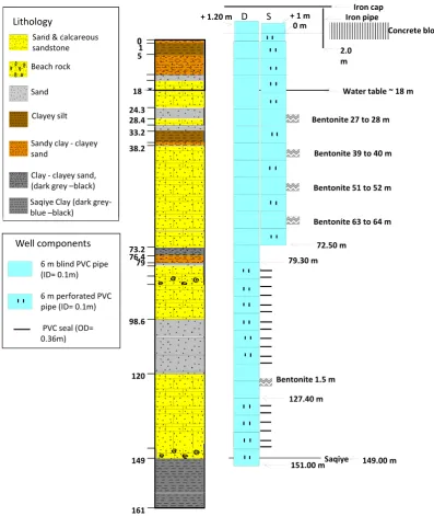
At the research site, extensive and intensive contamination of the unsaturated zone and groundwater with chlorinated or-ganic compounds and heavy metals has been reported (Ro-nen et al., 2005; Graber et al., 2008). The deep observa-tion well was drilled to explore the vertical distribuobserva-tion of contaminants at the center of the plume. The drilling re-vealed a 6-m thick clayey bed between 73 and 79 m below
ground level (m b.g.l.) (Fig. 2). Clayey beds (lenses) at these depths in this part of the aquifer are usually of continental origin and may be discontinuous over short distances (Ecker, 1999). Nevertheless, some studies have shown that this type of beds can create effective hydraulic separation (e.g. Nativ and Weisbrod, 1994). At the monitoring location, the full saturated thickness of the aquifer is∼130 m from the water table to the bottom confining Saqiye Group clays (Figs. 1 and 2). The monitoring well was drilled with a percussion tool and no drilling mud. It was designed to ensure reliable deep MLS by inserting bentonite and PVC seals into the sand-pack between and within perforated sections (Fig. 2). Two sepa-rate pipes, one tapping the deep part of the aquifer between 79 and 149 m b.g.l. (D, Fig. 2), and one tapping the shallow part of the aquifer between 18 and 72 m b.g.l. (S, Fig. 2), were installed in the borehole to avoid cross-contamination between the two parts of the aquifer.
2.2 MLS campaigns and chemical analyses
Groundwater samples were obtained using previously de-scribed passive MLS methodology (Ronen et al., 1986; Laor et al., 2003; Kurtzman et al., 2011). Briefly, each sampling unit consists of an individual stainless steel cylindrical dial-ysis cell (150 ml); the sampling units can be attached in a modular fashion, connected to each other with a chain. Each unit has a stainless steel ring into which the dialysis cell is in-serted. The dialysis cells are confined between flexible Viton seals that fit into the inner diameter of the well screen, creat-ing a 12-cm samplcreat-ing interval per cell. Before the chain of passive samplers is lowered into the well, the cells are filled with distilled water and closed on both sides with dialysis membrane (Versapor membrane, PALL corporation, 0.2 µm) crimped in a PVC hoop with a Viton O-ring.
Two multilevel profiles were obtained in the observation well. In the first sampling campaign (MLS1), the chain of sampling cells was deployed on 15 July 2008 and re-trieved on 10 August 2008. In the second sampling campaign (MLS2), the cells were deployed on 5 February 2009 and re-trieved on 1 June 2009. The retrieval date was regarded as the sampling date because the equilibration time of the dialysis cell with well water is short relative to the residence time of the cells in the well (∼48 h, Netzer et al., 2011). The mini-mum residence time required to ensure resumption of normal flow conditions has been estimated at 3 weeks (Netzer et al., 2011).
Observation
Well (b)
Israel
33oN
35oE (a)
‐
Coastal
Aquifer
West Bank
31oN
32oN
0 25 50 KM
Distance from coastline (km) Clay
Clay and silt Sand and
sandstone
Fig. 1. (a) Location map of the Israeli Coastal Aquifer (green). A cross section (red line) through the Tel Aviv metropolitan area is shown in (b). (b) East-west cross section of the aquifer, and the location of the observation well.
of 6 N HCl and 3 drops of concentrated HNO3, respectively.
The samples were stored at 4◦C until analysis, which was performed within 10 days.
Major anions were determined by ion chromatography (Dionex, Eluent Generator ICS-2500), major cations by ICP-MS (Thermo Jarrell, Ash-61) for MLS1, and by ICP OES (Varian, 720-ES) for MLS2, and trace elements were de-termined by ICP-MS. Bicarbonate (HCO−3)was determined by potentiometric titration with 0.002 N HCl using a Ra-diometer Titralab titrator. VOCs were determined by GC/MS headspace after addition of internal standard and 1:5 dilution (Netzer et al., 2011) using a Combi PAL Auto sampler (CTC Analytics), a 6890N network GC system (Agilent Technolo-gies) and a 5973 network Mass Selective Detector (Agi-lent Technologies). Dissolved organic carbon (DOC) (MLS2 only) was analyzed by Formacs TOC analyzer after sample acidification to pH 3.5 and air bubbling for 2 min. Chemi-cal analyses were performed at the laboratories of the Agri-cultural Research Organization, Israel, and the Israel Water Authority.
Two types of error can affect the determined concentra-tions: analytical and retrieval. Retrieval errors are unique to the specific deep MLS setting reported here, and may be significant in deep samples due to the time it takes to retrieve the deep dialysis cells. During retrieval, these cells may be in contact for short times (up to 75 min for the deepest samples, Ronen et al., 2010) with water that is not from the interval they sampled. Examples of total relative errors (sum of an-alytical and retrieval errors) are 2 to 12 % for Cl− and 12 to 21 % for trichloroethylene (TCE), where the higher errors are for the deeper samples (Ronen et al., 2010). In this re-port however, interpretations were focused on concentration differences with depth and time that were significantly larger than these errors.
2.3 Groundwater head and EC measurements
Head was measured in the deep (D) and shallow (S) pipes of the observation well (Fig. 2) 25 times between April 2008 and October 2009. A combined water level-temperature-conductivity logger (LTC, Solinst®) was inserted between Viton seals (similar to one interval of the MLS apparatus) and deployed at different depths (19, 20 and 31.5 m b.g.l.). The confined vertical length between the two seals was 35 cm. Water level, temperature and EC were recorded every 30 min. 2.4 Principal component analysis (PCA)
[image:3.595.91.503.70.230.2]Iron pipe Iron cap + 1 m
+ 1.20 m
0 m Concrete block
D S
Legend Legend
S d d l Legend Legend
S d d l Lithology
S d & l 0
1 5
18
24.3 28.4
Water table ~ 18 m 2.0
m
Bentonite 27 to 28 m Sand and calcareous
sandstone, yellow
Beach rock
Sand
Clay, brown Sand and calcareous sandstone, yellow
Beach rock
Sand
Clay, brown
Sand & calcareous
sandstone
Beach rock
Sand
Clayey silt
33.2
38.2
Bentonite 51 to 52 m Bentonite 39 to 40 m Clayey sand-sandy clay,
light brown-orange
Organic clayey sand, dark brown-black
Clay, dark grey-black, with shells
Clayey sand-sandy clay, light brown-orange
Organic clayey sand, dark brown-black
Clay, dark grey-black, with shells
Sandy clay ‐clayey
sand
Clay ‐clayey sand,
(dark grey –black)
Saqiye Clay (dark grey‐
blue –black)
73.2 76.4 79
Bentonite 63 to 64 m
79.30 m 72.50 m Well components
6 m blind PVC pipe
(ID= 0.1m)
6 m perforated PVC
pipe (ID= 0.1m)
98.6
120
127.40 m Bentonite 1.5 m
pipe (ID 0.1m)
PVC seal (OD=
0.36m)
149 149.00 m
151.00 m 127.40 m
Saqiye
[image:4.595.94.492.62.534.2]161
Fig. 2. Lithological log and perforation details of the observation well used for sequential multilevel sampling (MLS). D – pipe perforated against the deep subaquifer (79–149 m); S – pipe perforated against the shallow subaquifer (18–72 m); all depths are relative to ground level.
3 Results
3.1 MLS profiles
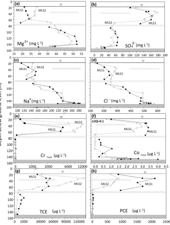
Profile pairs (MLS1 and MLS2) of eight representative chemical variables are presented in Fig. 4. The main charac-teristics of each chemical profile over the 130-m thick aquifer were preserved in both sampling events (Fig. 4). These gen-eral profile traits can be classified into five characteristic types: (a) concentrations generally increase with depth (e.g.
19 m
wt
MLS 2
19 m
wt
MLS
1
MLS
2
31.2 m
35 m
43 m
55m
145.7 m 47.5m
59.5 m 31.2 m
32 m
45.3 m
57.4 m
146 m
79.4 m
102.3 m 95.63 m
146.8 m
147.4 m 70.3 m
89.1 m
146.2m 67.2 m
84.2 m
102 m 95 m
147 m
147.5 m 70.3 m
114.3 m
130.1 m
140 m
147.8 m
148.40 m
144 m 142 m 114 m
130 m
140 m
148 m
148.5 m
145.7 m
148.45 m 144 m 146 m
[image:5.595.94.500.62.455.2]148.5 m
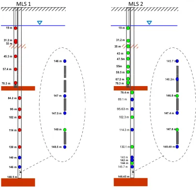
Fig. 3. Depth in meters below ground level (m b.g.l.) showing the positioning of the multilevel sampling (MLS) units in the two campaigns. Blue – 1 cell per depth (major ion and trace element analysis), green – 2 cells per depth and red – 3 cells per depth (major ion, trace element and volatile organic compound analyses). The dotted inset denotes details of the MLS below 145 m. Gray rectangles resemble weights that were inserted in the bottom of the chain of sampling cells to lead it down the well.
Despite the general similarities in chemical trends in the MLS1 and MLS2 profiles, a detailed examination revealed distinct differences between them. The most pronounced difference was the upward vertical shift of the boundary be-tween concentrations typical to the upper part of the aquifer and concentrations typical to the lower part of the aquifer for many of the chemical variables (e.g. Mg2+, SO2−
4 , Cr, Co,
TCE, and PCE, Fig. 4a, b, e–h). In MLS1, the boundary was consistent with stratigraphy, falling between the sam-pling depths of 70.3 and 84.2 m b.g.l., the interval that con-tains the 6-m thick clayey layer (Fig. 2), with Cr being the only exception. In MLS2, this hydrochemical boundary ap-peared to lie between 59.5 and 67.2 m b.g.l., i.e. within the upper sandy subaquifer (Figs. 3 and 4a, b, e–h).
Whereas the temporal shift in the hydrochemical bound-ary between the shallower and deeper waters was not seen in the Na+ and Cl− profiles (Fig. 4c and d), there was a clear change in the depth of the highest concentration gra-dients within the deep subaquifer. In MLS1, they occurred in the 84–96 m interval whereas in MLS2, they occurred be-tween 102 and 114 m (Fig. 4c and d). These large concen-tration gradients in the 102–114 m interval, which were ob-served only in MLS2, have also been noted for other vari-ables (NO−3, Br−, B; Ronen et al., 2010), and are clearly depicted in the PCA (Sect. 3.3).
3.2 Groundwater head and EC measurements
MLS2 MLS1
(a) (b)
MLS1 MLS2
100 80 60 40 20 0
0 20 40 60 80 100 120 140 160 180 200
SO422‐(mg L‐1)
MLS1 40
20 0
MLS2 MLS1
(c) (d)
15 20 25 30 35 40 45 50 55
Mg2+(mg L‐1) 160
140 120 100
u
nd
lev
el
(m)
Cl‐(mg L‐1) )
MLS2 MLS1
Na+(mg L‐1) Organic clay
160 140 120 100 80 60 40
Depth
below
gr
o
u 100 120 140 160 180 200 220 240 260 280 100 200 300 400 500 600
100 80 60 40 20 0
MLS2
MLS1
MLS1 MLS2
LOQ=0.1
(e) (f)
0 1000 2000 6000 12000
160 140 120
CrTotal
0.0 0.5 1.0 1.5 2.0 2.5 3.0 3.5 4.0 4.5
CoTotal
40 20 0
MLS1
MLS2 MLS2 MLS1
(g) (h)
(µg L‐1)
(µg L‐1)
0 1000 30000 60000 90000 120000 160
140 120 100 80 60
TCE
0 500 1000 1500 2000 2500
PCE
[image:6.595.133.468.64.506.2](µg L‐1) (µg L‐1)
Fig. 4. Representative deep aquifer profiles obtained in sequential sampling campaigns. (a–d) major ions; (e, f) trace elements and (g, h) volatile organic compounds (VOCs). MLS1 (circles) obtained 10 August 2008; MLS2 (squares) obtained 1 June 2009. Saqiye Group clay in gray is the bottom aquifer boundary and clayey layers around 35 and 75 m depth are illustrated with dashed lines (Fig. 2). LOQ (f) – limit of quantification.
than that measured in the shallow pipe (S, Fig. 2) in 11 out of 12 measurements (∼97 % of the time, Fig. 5). The dif-ference between the overall head in the deep subaquifer and the head in the shallow subaquifer during the 295-day pe-riod ranged between−2 and 27 cm (Fig. 5). These data are suggestive of upward flow from the deep to shallow parts of the aquifer during the time interval between the two sampling dates. However, this is not a definitive interpretation, as these head measurements reflect the overall head in the tapped part of the aquifer rather than the specific head at a given point in the screened interval. Therefore, we can only conclude that,
looking over the entire width of the aquifer during this pe-riod, the vertical component of flow was more upward than downward; we cannot draw any conclusion as to the prevail-ing flow at any specific depth.
0.7 0.8
m
asl)
0.3 0.4 0.5 0.6
D
MLS2 1/6/09
H
ydraulic
head (
m
S
MLS1 10/8/08
11/10/08
1/6/09 10/8/08
12/9/09 27/3/09
[image:7.595.311.541.62.275.2]26/4/08
Fig. 5. Elevation of the hydraulic heads observed in the deep aquifer in gray (measured in pipe D, Fig. 2) and the shallow sub-aquifer (measured in pipe S, Fig. 2). The dotted vertical lines de-note the retrieval dates of MLS1 and MLS2. m a.s.l. – meters above sea level.
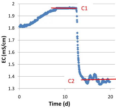
2 months of observations in which the LTC probe was po-sitioned at the three depths (∼3 weeks per depth). Head and temperature, measured simultaneously, did not show any such contemporaneous discontinuities. Hence, the change can only be explained by lateral flow of a fresher water body through the monitored section. Changes in concentration in the packed-off section during this passage are caused by wa-ter from the inwa-terval with concentrationCleaving the inter-val and new water with lower concentrationC2 entering the interval (Eq. 1, Fig. 6).
dC dt = −
Q
V(C−C2) (1)
where t is time (T), Q is flow rate through the interval (L3T−1)andV is the volume of the packed-off section (mi-nus the probe volume) (L3). Equation (1) is similar to mass balance equations used for the interpretation of dilution tests (e.g. Brouy`ere et al., 2005; Kurtzman et al., 2005). The solu-tion of Eq. (1) for our case is:
ln(C−C2 C1−C2)= −
Q
V(t−t1) (2)
whereC1 andt1 are the concentration and time, respectively, at the beginning of the concentration change (Fig. 6). Plot-ting the left-hand side of Eq. (2) againstt−t1 enables cal-culation of−Q/V (the slope). SinceV is known,Qcan be determined. Groundwater specific discharge−q (L T−1)is derived by Eq. (3).
q= Q
LsDsα
(3) whereLs andDs are the section’s length and diameter,
re-spectively (L) andα (−) is a factor correcting for the con-vergence of the natural aquifer flow toward the well (α= 2 is
1.8 1.9 2
C1
1.4 1.5 1.6 1.7
EC
(m
S/
cm
)
C2
1.30 10 20
t (d)
[image:7.595.54.282.64.233.2]Time
(d)
Fig. 6. Electrical conductivity (EC) monitored in a 35 cm packed-off section of the observation well at 31.5 m below ground level. Note the sharp change in EC on day 12, suggesting a relatively fresh water body flowed through the monitored section.
widely accepted and used here; e.g. Pitrak et al., 2007). This analysis resulted in q∼40 m yr−1. If we use an effective porosity of 0.25 for this aquifer (e.g. Assouline and Shavit, 2004), we have a groundwater velocity (v)in the neighbor-hood ofv∼150 m yr−1. This lateral velocity estimate sug-gests that some tens to hundred meters may laterally divide the water bodies sampled in MLS1 and MLS2. EC and chlo-ride concentration from the two MLSs show a significant lin-ear relation (R2= 0.76, P value<1×10⁻¹¹), hence the EC observations can be approximated as concentrations for the above calculations.
3.3 PCA of the sequential MLS profiles
In the following, results and interpretations concerning the main sources of variability, and water-body classification will be discussed using the projections of variables (chem-icals) and cases (depths) on the plane of the first and second PCs (Fig. 7). The correlation of a variable with a PC is the value of that PC component in the variable projection onto the plane of the PCs. For example, in Fig. 7a we see that in the PCA of MLS1, the correlation of Ca2+with PC1 (hori-zontal axis) is 0.84 and with PC2 (vertical axis), 0.03.
(b) MLS2 i bl j t d PC1 PC2 l
Projection of the variables on the factor-plane ( 1 x 2)
K Mg
C HCO3
TDS Al Be
Pb Sr 0.5 1.0 19 % K Mg C HCO3
TDS Al Be
Pb Sr
9%
(a) MLS1, variables projected on PC1-PC2 plane
9% Sr Mg Mg Sr HCO3 0.5 1.0 Mg Sr HCO3
(b) MLS2, variables projected on PC1-PC2 plane
Na
Ca
Cl SO4NO3
Br As B Ba Co Cr Mn Ni Se U -1.0 -0.5 0.0 F act or
2 : Na
Ca
Cl SO4NO3
Br As B Ba Co Cr Mn Ni Se U
PC 2: 1 Na, Cl PC 2: 1
SO4 NO3 Na K Ca Cl Br SO4 NO3 TDS B Be Ba Co Cr Li Mn U DOC -1.0 -0.5 0.0 Na K Ca Cl Br SO4 NO3 TDS B Be Ba Co Cr Li Mn U DOC Ca DOC Cr U Mn Ba Li Br Na
(d) MLS 2, cases projected on PC1‐PC2 plane
-1.0 -0.5 0.0 0.5 1.0
Factor 1 : 55%PC 1: 55%
-1.0 -0.5 0.0 0.5 1.0
PC 1: 62%
(c) MLS1, cases projected on PC1-PC2 plane
84.2 95 102 114 130 140 84.2 95 102 114 130 140 3 intermediate 79.4 89 1 79.4 89 1 4 intermediate 19
31.23245.3 57.4 70.3 146 147 147.5 148 19
31.23245.3 57.4 70.3 146 147 147.5 148
PC 2: 19%
2 1 0 -1 -2 -3
bottom top 19
43 47.5
55 59.5
67.2 70.389.195.6
102.3 114.3 130.1140 142 144 145 7 146.2 146.8 147.4147.8 19 43 47.5 55 59.5 67.2 70.389.195.6
102.3 114.3 130.1140 142 144 145 7 146.2 146.8 147.4147.8 67.2 70.3
PC 2: 19%
2 1 3 0 -1 bottom
top 147.4 147.8
146.8
148.5 148.5
PC 1: 55%
2 4 6
0 -2 -4 -6
-4 3531.2
43 145.7144
148.4 31.2 3543 144 145.7 148.4
2 4 6
0 -2 -4 -6 -2
PC 1: 62%
31.2 145.7
[image:8.595.97.497.65.454.2]35
Fig. 7. Principal component analysis (PCA) of the multilevel sampling (MLS) campaigns. Variables (a, b) and cases (c, d) are projected on the plane of the first two principal components. Cases are labeled by the sampling depth in meters below ground level (m b.g.l.). Top, intermediate and bottom groups of cases are distinct. Oxidation states of ions were omitted for graphical simplicity.
correlations with PC1, but with the opposite sign to that of the type (a) variables, in both MLS1 and MLS2 (Fig. 7a and b). These results suggest that PC1 in both PCAs is closely related to depth. Therefore the correlation of PC1 with depth (a type (a) variable), was calculated and found to be−0.97 in the PCA of MLS1 and 0.96 in the PCA of MLS2. PC1 ex-plains 55 % and 62 % of the variability in MLS1 and MLS2, respectively (Fig. 7a and b); hence, we can postulate that depth is the major controller of chemical variability in the profile. This can also be visualized in the distribution of cases (depths) along the PC1 axis. Cases of the bottom part of the aquifer are on one side of the PC1 axis, whereas cases from the top of the aquifer are on the opposite side of the axis, while cases from the intermediate depths are close to 0 on this axis (Fig. 7c and d).
relatively high positive correlation with PC2 in both MLS1 and MLS2 (Fig. 7a and b). The physical phenomenon that has a greater impact on PC2 is the abrupt change in concen-tration that was found for some variables near the bottom of the aquifer. These variables include metals such as Mn2+, Co, As (increase in concentration near the bottom) and ma-jor ions Mg2+, HCO−3, SO24−(decrease in concentration near the bottom) (Ronen et al., 2010). These variables will have a relatively high correlation with PC2 if the abrupt change in concentration near the bottom of the aquifer is counter to the variables’ general trend with depth, hence forming a non-monotonous profile (e.g. compare profiles and PC2 correla-tions of Mg2+and SO24−in Figs. 4a, b, 7a and b). In light of this analysis of PC2 (19 % of variability in both MLS1 and MLS2), it can be concluded that the second important control over chemical variability in the profile is the different hydro-chemical conditions that prevail at the bottom of the aquifer. Both MLS1 and MLS2 case projections show three dis-tinct groups that are consistent with depth (Figs. 3, 7c and d). The clear distinction of three vertically separated water bodies in the PCAs of the MLS1 and MLS2 chemical data is the most significant outcome of the PCA for aquifer dynam-ics characterization. Hereafter, these three water bodies are denoted as top, intermediate and bottom (Fig. 7c and d).
A significant difference between the PCAs of MLS1 and MLS2 was that some sampling depths were in different wa-ter bodies: depths 67 and 70.3 m b.g.l. were in the top wawa-ter body in MLS1 and were shifted to the intermediate one in MLS2. Depths 114, 130 and 140 m b.g.l. were in the in-termediate water body in MLS1 and in the bottom water body (or at least much closer to it) in MLS2 (Fig. 7c and d). The boundary between the top and intermediate water bodies was between 70 and 84 m in MLS1 (consistent with stratigraphy, Fig. 2), whereas in MLS2, this boundary lay tween 59 and 67 m b.g.l. It also appears that the boundary be-tween the intermediate and bottom water bodies shifted from between 140 and 146 m b.g.l. in MLS1 to between 102 and 114 m b.g.l. in MLS2 (Fig. 7c, d). These changes in the posi-tion of the boundaries between the chemically different water bodies that could be obtained, to some extent, by exploring the profiles of MLS1 and MLS2 (Fig. 4) became sharper with the PCA (Fig. 7). A discussion of the aquifer dynamics that may have caused these vertical shifts of water-body bound-aries follows.
4 Discussion
4.1 Aquifer dynamics that can explain the change between MLS1 and MLS2
Two possible “end member” flow regimes near the observa-tion well were examined. Assuming a 1-D vertical system and neglecting changes in the concentrations of major and trace elements due to reactions during the 295 days between
(b) (a)
Observation well
20
30
40
MLS2 MLS1
50
60
70
80
L H
m
bgl)
90
100
110
120
L H
Depth
(m
Flow
120
130
140
150
[image:9.595.311.543.64.278.2]Time
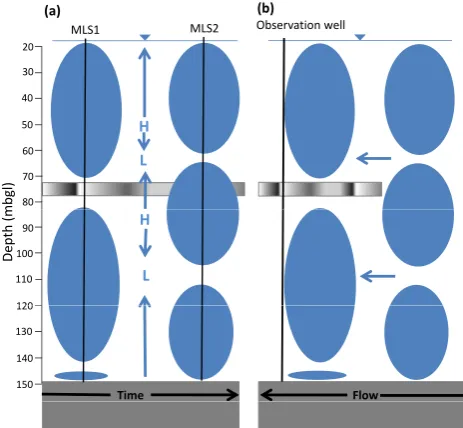
Fig. 8. Schematic representation of flow regime end members near the observation well. Blue ellipses present the water bodies inferred in the PCA of MLS1 (left) and MLS2 (right). (a) Vertical-dominant flow regime during the time between samplings that might support the differences in the vertical distribution of the water bodies ob-served in the two campaigns. “L” and “H” represent relatively low and high hydraulic heads, respectively. (b) Lateral flow of water bodies passing through the observation well as an alternative expla-nation of the differences. An arbitrary snapshot before MLS1 sam-pling date is presented. Note that MLS2 water bodies are assumed to originate from an area where the clayey bed at 73–79 m b.g.l. is absent.
MLS1 and MLS2, a vertical flow regime can be hypothe-sized to explain the changes in the vertical distribution of the three water bodies obtained by the PCA (Figs. 7c, d and 8a) as follows. The water from the bottom of the aquifer flowed upward to form a larger water body which is a mix of the previous bottom water and the deeper part of the previous intermediate water (Figs. 7d and 8a). The upper part of the intermediate water body was pushed up over the intermediate clay. Relatively low heads at∼65 m depth might have trig-gered the upward flow in the column which moved the high chemical gradients over the clay into the shallow subaquifer (Figs. 4a, b, f–h and 8a). Within the upper section, it looks as though there was also upward movement, raising the upper subaquifer’s peaks in MLS2 (Figs. 4b–e, g and 8a).
Evidence of lateral flow of distinct water bodies through the monitoring well at 31.5 m b.g.l. (∼13 m below the water table), which was observed by EC monitoring (Fig. 6), sup-ports the lateral flow hypothesis. Water parcels with differ-ent chemical characteristics on a smaller scale (0–2 m below the water table) at a polluted site in the same aquifer were reported by Ronen et al. (1987). A lateral flow regime sug-gests that the intermediate water body in MLS2 was formed in a place in the aquifer where the 73–79 m b.g.l. clayey layer is absent; after flowing laterally into the clay-divided area of the aquifer, it exists both on top of, and below the clay layer (Fig. 8b). As mentioned in the site description (Sect. 2.1), clayey layers at these depths in this part of the aquifer are usually of continental origin can often be discon-tinuous over short distances. Therefore, the lateral flow ex-planation makes more sense than fast vertical flow across the clayey layer.
Further indirect evidence supporting the lateral flow “end member” is the lack of mass conservation within the water bodies: such mass conservation would be expected if we assume that the differences between the profiles occurred due to upward flow. Looking at the industrial-contaminant profiles (Fig. 4e, g and h), we observe large differences in concentrations between the top and intermediate water bodies in both MLS1 and MLS2, while the contaminant concentrations in the intermediate and bottom water bodies are similar. Focusing on the top water body, we see that whereas the mass of TCE and Cr increased significantly from MLS1 to MLS2, the mass of PCE decreased (Fig. 4e, g and h). High TCE concentrations increased from∼50 000 to∼120 000 µg l−1, whereas PCE concentrations decreased from ∼1800 to ∼700 µg l−1, such that these changes can-not be explained by degradation of PCE to TCE. It is more likely that MLS1 and MLS2 sampled different water bodies with different contaminant characteristics due to their differ-ent lateral origin and history.
4.2 Implications for sites with industrial contamination
One of the most practical outcomes of this work is the idea that by sampling a single monitoring well via several consec-utive MLSs, it is possible to arrive at a certain understanding of the spatial character of the subsurface contamination. This is because ambient water flow passes through the monitoring well and can be characterized. This information is very valu-able in sites within cities where construction of monitoring wells is not a trivial undertaking, as it can be used to develop a site-specific monitoring network and remediation plan. For example, at the study site, a distinct difference between con-tamination extent in the upper and lower parts of the aquifer was apparent. In the upper part of the aquifer, the presence of distinct water bodies having limited horizontal and vertical extents suggests that the spacing between monitoring wells should be relatively small (on the order of tens of meters). In the lower part of the aquifer, contamination levels are much
lower, such that the density of monitoring wells there can also be significantly lower.
Differences in contamination characteristics between the water bodies and their large degree of mobility can also impact both the selection of remediation technologies and cleanup progress. At the study site, for instance, remedia-tion methods would need to be able to handle contaminants whose concentrations vary both spatially and temporally due to the movement of distinct water bodies. Apparent reme-dial progress may not be linear in such a system, not because the method does not work, but because background concen-trations are changing due to the movement of distinct water bodies.
5 Summary and conclusions
Acknowledgements. This study was financed by the Israel Water Authority. The presented conclusions are those of the authors of this study.
Edited by: P. Grathwohl
References
Angelone, M., Cremisini, C., Piscopo, V., Proposito, M., and Spaziani, F.: Influence of hydrostratigraphy and structural set-ting on the arsenic occurrence in groundwater of the Cimino-Vico volcanic area (central Italy), Hydrogeol. J., 17, 901–914, 2009.
Assouline, S. and Shavit, U.: Effects of management policies, in-cluding artificial recharge, on salinization in a sloping aquifer: The Israeli coastal aquifer case, Water Resour. Res, 40, W04101, doi:10.1029/2003WR002290, 2004.
Brouy`ere, S., Carabin, G., and Dassargues, A.: Influence of injec-tion condiinjec-tions on field tracer experiments, Ground Water, 43, 389–400, 2005.
Cherry, A., Parker, B. L., and Keller, C.: A new depth-discrete multilevel monitoring approach for fractured rock, Ground Water Monit. R., 27, 57–70, 2007.
Ecker, A.: Atlas-selected geological cross sections and subsurface maps in the coastal aquifer of Israel, Report No. GSI/18/99, 151 pp., 1999 (in Hebrew).
Graber, E. R., Laor, Y., and Ronen, D.: Megasite aquifer contamina-tion by chlorinated-VOCs: A case study from an urban metropo-lis overlying the coastal plain aquifer of Israel, Hydrogeol. J., 16, 1615–1624, doi:10.1007/s10040-008-0366-2, 2008.
Hendry, M. J., Barbour, S. L., Zettl, J., Chostner, V., and Wasse-naar, L. I.: Controls on the long-term downward transport ofδ2H of water in a regionally extensive, two-layered aquitard system, Water Resour. Res., 47, W06505, doi:10.1029/2010WR010044, 2011.
Issar, A.: Stratigraphy and paleoclimates of the Pleistocene of cen-tral and northern Israel, Palaeogeogr. Palaeocl., 29, 261–280, 1980.
Kurtzman, D., Nativ, R., and Adar, E.: The conceptualization of a channel network through macroscopic analysis of pumping and tracer tests in fractured chalk, J. Hydrol., 309, 241–257, 2005. Kurtzman, D., Netzer, L., Weisbroad, N., Graber, E. R., and Ronen,
D.: Steady-state homogenous approximations of vertical velocity from EC profiles, Ground Water, 49, 275–279, 2011.
Laor, Y., Ronen, D., and Graber, E. R.: Using a passive multilayer sampler for measuring detailed profiles of gas-phase VOCs in the unsaturated zone, Environ. Sci. Technol., 37, 352–360, 2003. Moore, P. J., Martin, J. B., and Screaton, E. J.: Geochemical and
statistical evidence of recharge, mixing, and controls on spring discharge in an eogenetic karst aquifer, J. Hydrol., 376, 443–455, 2009.
M¨uller, K., Vanderborght, J., Englert, A., Kemna, A., Huisman, J. A., Rings, J., and Vereecken, H.: Imaging and character-ization of solute transport during two tracer tests in a shal-low aquifer using electrical resistivity tomography and multi-level groundwater samplers, Water Resour. Res., 46, W03502, doi:10.1029/2008WR007595, 2010.
Nativ, R. and Weisbrod, N.: Hydraulic connections among sub-aquifers of the coastal plain aquifer, Israel, Ground Water, 32, 997–1007, 1994.
Netzer, L., Weisbrod, N., Kurtzman, D., Nasser, A., Graber, E. R., and Ronen, D.: Observations on vertical variability in groundwa-ter quality: Implications for aquifer management, Wagroundwa-ter Resour. Manag., 25, 1315–1324, 2011.
Pitrak, M., Mares, S., and Kobr, M.: A Simple borehole dilution technique in measuring horizontal ground water flow, Ground Water, 15, 89–92, 2007.
Ronen, D., Magaritz, M., and Levy, I.: A multi-layer sampler for the study of detailed hydrochemical profiles in groundwater, Water Res., 20, 311–315, 1986.
Ronen, D., Magaritz, M., Gvirtzman, H., and Garner, W.: Mi-croscale chemical heterogeneity in groundwater, J. Hydrol. , 92, 173–178, 1987.
Ronen, D., Graber, E. R., and Laor, Y.: Volatile organic compounds in the saturated-unsaturated interface region of a contaminated phreatic aquifer, Vadose Zone J., 4, 337–344, 2005.
Ronen, D., Netzer, L., Nasser, A., Weisbrod, N., Kurtzman, D., and Graber, E. R.: Assessment of aquifer contamination in the Nahalat Itzhak area – Tel Aviv: Phase iii – final report, Israel Water Authority, 2010.
StatSoft Inc.: Electronic statistics textbook, avail-able at: http://www.Statsoft.Com/textbook/ principal-components-factor-analysis/?Button=1, StatSoft, Inc., Tulsa, OK, USA, 2011.
Stetzenbach, K. J., Farnham, I. M., Hodge, V. F., and Johannesson, K. H.: Using multivariate statistical analysis of groundwater ma-jor cation and trace element concentrations to evaluate ground-water flow in a regional aquifer, Hydrol. Process., 13, 2655– 2673, 1999.
Williams, B. A. and Chou, J. C.: Characterizing vertical con-taminant distribution in a thick unconfined aquifer, Han-ford site, Washington, USA, Environ. Geol., 53, 879–890, doi:10.1007/s00254-007-0700-3, 2007.