CFD simulation of vortex induced vibration of a bluff body structure by ANSYS fluent

(1)

CFD SIMULATION OF VORTEX-INDUCED

VIBRATION OF A BLUFF BODY STRUCTURE BY

ANSYS FLUENT

ABDUL HALIM BIN ABDUL RAHMAN

A project report submitted in partial

fulfillment of the requirement for the award of the

Degree of Master of Mechanical Engineering

Faculty of Mechanical and Manufacturing Engineering

Universiti Tun Hussein Onn Malaysia

(2)

Abstract

Vortex-induced vibration is a vibration phenomenon which occurred to the bluff body structure either on the ground or sea underneath. The investigations of

the effect of flow velocity on the transverse vibration of bluff body were done

to determine the vortex shedding frequency for each of the analyses. Besides it

was also to investigate the flow velocity and pressure loss in the time response.

Despite the investigation made by other researchers, a study on a very high

turbulence Reynolds number, were still blurred unknown. In response to this

problem, this study is purposely to investigate at a very high Reynolds number

and simulated through ANSYS Fluent software’s which started from a minimum

of 70 000 Reynolds number and increased to the maximum of 350 000 Reynolds number. A one meter in diameter of cylindrical aluminium was used for the

study where the velocity was in cross-flow direction. From the simulated results,

it could be seen the fluid flow after the boundary layer was an asymmetric flow.

The Strouhal number seems to be decreased by the increase of Reynolds number

while the frequencies were increased with the increased of Reynolds number.

(3)

Abstrak

Getaran disebabkan vorteks (VIV) adalah satu fenomena getaran yang berlaku kepada struktur badan tumpul samada di tanah atau di bawah laut. Kajian

ter-hadap kesan halaju aliran pada getaran melintang badan tumpul telah dilakukan

untuk menentukan frekuensi penumpahan vorteks bagi setiap analisis. Selain itu

tujuan penyelidikan ini juga dalah untuk menyiasat halaju aliran dan

kehilan-gan tekanan didalam tindak balas masa. Walaupun terdapat penyelidikan yang

dibuat oleh penyelidik lain, kajian mengenai pergolakan nombor Reynolds yang

sangat tinggi, masih kabur dan tidak diketahui. Untuk menjawab

permasala-han ini, kajian ini bertujuan untuk menyiasat dengan nombor Reynolds yang

sangat tinggi melalui simulasi perisian ANSYS Fluent yang bermula dari mini-mum 70 000 nombor Reynolds dan meningkat kepada maksimini-mum 350 000 nombor

Reynolds.. Satu selinder aluminium yang bergaris pusat satu meter telah

digu-nakan dalam kajian ini di mana halaju aliran adalah dalam arahan merentas

selin-der. Hasil dari keputusan simulasi, dapat dilihat cecair yang mengalir melepasi

lapisan sempadan adalah aliran tidak simetri. Nombor Strouhal kelihatan

menu-run apabila nombor Reynolds meningkat, manakala frekuensi pula meningkat

dengan peningkatan nombor Reynolds.

(4)

List of Figures

2.1 Cylinder arrangement in the wind tunnel 9

3.1 Schematic diagram of the flow field around circular cylinder [7] 13

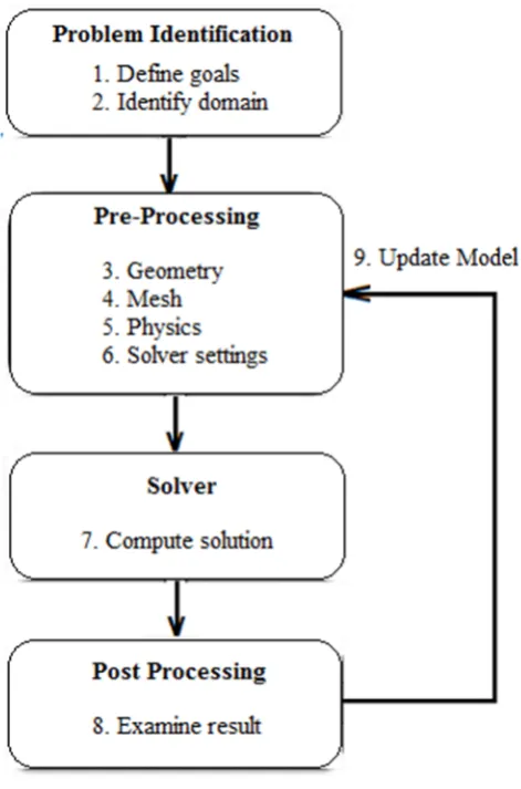
3.2 Steps Performed in CFD 19

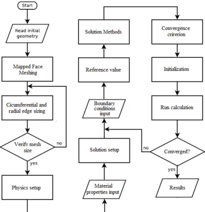
3.3 Flowchart of Methodology 21

4.1 Trending line validation between present study and Simmons 23 4.2 Contours of Velocity Magnitude at Re=70000 24

4.3 Vectors of Velocity Magnitude at Re=70000 24

4.4 Contours of Velocity Magnitude at Re=150000 24

4.10 Contours of Velocity Magnitude at Re=300000 26 4.11 Vectors of Velocity Magnitude at Re=300000 27

4.14 Contours of Vorticity Magnitude at Re=70000 28

4.15 Vectors of Vorticity Magnitude at Re=70000 28

4.19 Vectors of Vorticity Magnitude at Re=200000 30 4.20 Contours of Vorticity Magnitude at Re=250000 30

(7)

xi

4.26 Vectors of Pressure Coefficient at Re=70000 33 4.27 Pressure Coefficient around cylinder at Re=70000 33

4.28 Vectors of Pressure Coefficient at Re=150000 33

4.29 Pressure Coefficient around cylinder at Re=150000 34

4.35 Pressure Coefficient around cylinder at Re=300000 36 4.36 Vectors of Pressure Coefficient at Re=350000 36

4.38 Strouhal Number vs Reynolds Number 38

4.39 Strouhal Number at Re=70000 38

4.45 Frequencies of Vortex Shedding vs Reynolds Number 41

4.46 Period vs Reynolds Number 41

B.1 Frequency at 70 000 Re, extracted directly from analysis figure 51

(8)

List of Tables

4.1 Pressure Coefficient for different Reynolds Number 37

4.2 Strouhal Number at different Reynolds Number 37

4.3 Calculated of Frequencies of Vortex Shedding and Period 40

A.1 Data of Analysis 47

(9)

List of Appendices

A Frequency of Vortex Shedding 47

B Figure of Frequency 49

(10)

List of Symbols

2D Two-dimensional

3D Three-dimensional

Ã Diffusion coefficient

Δt Time-step

ε Turbulence dissipation rate μ Dynamic viscosity (Ns/m2) ρ Fluid density (kg/m3) ω Specific dissipation rate

Cµ Empirical constant

Cd Drag coefficient

CFD Computational Fluid Dynamics

CWT Cooperative Wind Tunnel

D,d Diameter (m)

DNS Direct Numerical Simulation

(11)

xv

f Frequency

F_o Vortex shedding frequency

FDM Finite Difference Method

FEM Finite Element Method

FIV Flow-Induced Vibration

FVM Finite Volume Method

I Turbulence intensity

k Kinetic energy

LES Large Eddy Simulation

Re Reynolds number

SST Shear Stress Transport

St Strouhal number

U Fluid velocity (m/s)

U∞ Free stream velocity

Uavg Mean flow velocity

(12)

Chapter 1 Introduction

This chapter discussed about the CFD Simulation of Vortex-Induced Vibration of

the Bluff Bodies Structure by ANSYS Fluent. The chapter consists of the

back-ground study, the problem statement, the objectives and the scopes of study. In

the background study, the reader is then introduced to the CFD’s Simulation,

the vortex-induced vibration (VIV), the bluff bodies and the ANSYS Fluent

soft-ware’s.

1.1 Background of Study

In designing of a structure or structures, vibration of a structure is an important

issue to encounter with. A structure could lead to a fatigue damage which is

caused by vibrations. The environmental loading, either on the ground such as

wind, or sea underneath such as waves and currents, are the main cause of the

vibration.

In recent years, the study of flow around a bluff body becoming an

impor-tant study, to investigate the effect of the flow induced vibration [1]. Its effect is

relevant in designing, an on the ground structures such as taller buildings, bridges

and other similar structures. Its effect also relevant in designing sea underneath

structures such as pipelines and risers.

(13)

2

1.1.1 Vortex-Induced Vibration

Vibration phenomenon which occurs to the bluff body structure, either on the

ground or sea underneath could be regarded as vortex-induced vibration (VIV).

Previous researchers have been widely discussed in both detail and comprehensive

ways to understand the vortex-induced vibration mechanism from a bluff body [2,3].

As the flow passed a bluff body at a sufficiently large Reynolds number,

vortices would be shedding at the trailing edge of the body. A fluctuating lift

forced, was created due to the pressure difference on the side of the body surface

which eventually would create cross-flow vibrations.

The source of vibration was from the vortex formed that occurs after

the flow passed a bluff body structure. Large amplitude vibration phenomenon

would strike if the frequency of the vortex shedding and approaching the natural

frequency of the bluff body structure.

These large amplitudes vibration phenomena were also called lock-in [1].

This typed of fluid-structure interaction problem has been widely investigated

numerically and experimentally in the past.

1.1.2 Bluff Body

There were two types of shape’s structure which were that streamline shape and

non-streamline shape. The streamline shapes often called aerodynamic body

while the non-streamline shape often called bluff body.

As a result of its shape, a bluff body separated, flow over a substantial

part of its surface. An important feature of a bluff body flow is that there is a very

strong interaction between the viscous (significant to the frictional effect because

of the viscosity) and inviscid (ideal fluid that is assumed to have no viscosity)

regions [4,5]. Examples of bluff bodies include circular cylinders, square cylinders

(14)

3

1.1.3 Computational Fluid Dynamics (CFD)

CFD calculates numerical solutions to the equations governing fluid flow. As

opposed to flow around a streamlined body, bluff bodies were the structures with

shapes that significantly disturb the flow around them.

To model the fluid-structure interaction, the CFD software ANSYS

Flu-ent 14 was used to predict the results around cylindrical bluff body at each time

step. The cylindrical bluff body structured was tested at a difference Reynolds

number. The predicted results around the cylindrical bluff body are validated

through previous journals results.

1.2 Problem Statement

At low flow velocities, the fluid flow around the cylindrical bluff body acts as

a damper, limiting the amplitude of motion. The investigations of the effect of

flow velocity on the transverse vibration of bluff body were done to determine

the vortex shedding frequency for each of the analyses. Besides it was also done

to investigate the flow velocity and pressure loss in the time response.

However, as the flow velocity increased, the pressure and shear forces

also increased, which increased the net lift and drag forces on the cylindrical bar.

Eventually, at some critical velocity, the energy input from these external fluid

forces exceeds the structural damping and the amplitude of the cylindrical bluff

body vibration rises dramatically, particularly in the cross-flow direction. Despite

the investigation made by other researchers, a study on a very high turbulence

Reynolds number, were still blurred unknown.

In response to this problem, this study proposed to investigate several

options such as increasing the Reynolds number. The turbulence studied started

from a minimum of 70 000 Reynolds number and increased to the maximum of

350 000 Reynolds number.

1.3 Objective of the Study

(15)

4

1. To investigate the effect of flow velocity on the transverse vibration of bluff

body.

2. To determine the Strouhal number for each of the analyses.

3. To determine the vortex shedding frequency for each of the analyses.

1.4 Scopes of the Study

The scopes for this study were:

1. Aluminium cylindrical shape with one meter of diameter.

2. Shape is allow to move in cross-flow direction

3. Test at different Reynolds Number which were 70 000 Re, 150 000 Re, 200

000 Re, 250 000 Re, 300 000 Re and 350 000 Re.

(16)

Chapter 2 Literature Review

This chapter discussed about the work of past researchers. This chapter would

discuss about the Reynolds number, the Strouhal number, the effect of flow

ve-locity, the vortex shedding and the previous work of research. In the previous

research, several sub-topics will be discussed such as, the methodology, results

and discussion and finally the conclusion of previous research.

Fluid flowed behaviour could be analysed throughout the experiment and

empirical studies. To study the characteristics of the fluid flows, several tests had

been conducted. Differential equations and mathematical relations were used to

obtain new equations. Experimental and numerical method was always used as

the methods to investigate the fluid behaviour.

To solve the numerical equations, a program called Computational Fluid

Dynamics (CFD) was developed. Throughout the development of CFD, numbers of fluid problem were solved, although it was a complicated problem. Vortex

shedding was one example of the complicated problems, which need to be solved

computationally.

For many decades, vortex shedding from the bluff bodies has been always

a main subject that attracted many researchers to study and investigate. A high

tower building, for example, is the significance of the periodic unsteady fluid flows which passed from bluff bodies. Vibrations near the bluff body were produced

by the vortices which may be dangerous to the structure.

(17)

6

2.1 Reynolds Number

One of the very important non-dimensional numbers was the Reynolds Number

(Re) [3-9]. It is used in predicting flow patterns in different fluid flow situations.

The Reynolds numbers expresses the ratio of inertial (resistant to change or

mo-tion) forces to viscous (heavy and gluey) forces [2]. Reynolds numbers determines

dynamic similitude between two different cases of fluid flow.

Reynolds Number is given by the formula,

Re= ρUD

μ

(2.1)

whereρ is the fluid density (kg/m3), U is the velocity based on the actual across

area of the duct or pipe (m/s), D is the pipe diameter (m) and μ is the dynamic

viscosity (Ns/m2).

Besides that, Reynolds number also used to characterize different flow

regimes within a similar fluid, such as laminar flow or turbulent flow. Laminar

flow is characterized by smooth and constant fluid motion. Laminar flow occurs at

low Reynolds numbers, where viscous forces were the dominant. Turbulent flow

occurs at high Reynolds numbers and is dominated by inertial forces. Turbulent

flow produces chaotic eddies, vortices and other flow instabilities.

2.2 Strouhal Number

Another important non-dimensional number was the Strouhal number (St)

[4-9]. The Strouhal number is used to analyse the unsteady-state, oscillating flow

problems [10].

Strouhal number, defined as a ratio of inertial forces due to the

unsteadi-ness of the flow or local acceleration to the inertial forces due to changes in

velocity from one point to another in the flow field [10].

Strouhal Number is given by the formula,

St= f D

(18)

7

where f is the characteristic oscillation frequency, D is the characteristic

length and U is the velocity of the fluid.

2.3 Effect of Flow Velocity

Several factors such as force components, shedding frequency, Reynolds number,

material damping and structural stiffness of the cylinder, were the caused that

affected the vortices to generate [11].

As the Reynolds number increases, the amplitude as well as the frequency

of the velocity signals also increases. An increase in Reynolds number causes an

increase in the Strouhal frequency of a single bluff body and for a row of bluff

bodies [12].

2.4 Vortex Shedding

When shedding vortices (a Von Karman vortex street) exert oscillatory forces on

a cylinder in the direction perpendicular to both the flow and the structure, a

vortex-induced vibration (VIV) occurs [11].

When a solid and fluid interact, the instabilities appearing in flow fields

induce instabilities in the neighbouring solid structures [12]. Special emphasis is

required to analyse the VIV because vortex shedding and wake dynamics or flows passed bluff bodies were a complex flow problem [2, 12].

When cylinders with a bluff cross section, immersed in a free stream

with their axis perpendicular to the flow, they were susceptible to a range of

flow-induced vibration (FIV) phenomenon [13]. For circular cylinders, which do

not have a defined angle of attack, the phenomenon of VIV is more likely to

occur, which is due to periodic vortex shedding in the wake [13].

The periodic shedding was where a vortex was shedding from one side of

the body, and then a vortex of opposite sign was shedding from the other side of

the body and forms the Karman vortex street [13]. Large-amplitude oscillations

can occur in the resonance-type response when the vortex shedding frequency

(19)

8

also would change to match with the body oscillation frequency, which leading

to large, periodic oscillations.

2.5 Previous Research

Rahman et.al [14] investigates unsteady flow passed a circular cylinder using a

2D finite volume method with different Reynolds number.

Vijaya et.al [15] studied 2D unsteady flows of power-law fluids over a

cylinder. The study has been solved using a finite volume method based solver

FLUENT 6.3.

Mittal and Kumar [2] studied VIV on a pair of equal-size cylindrical

cylinders with two sets of arrangement, inline and staggered. The fixed cylinders

for the 2D simulation were simulated in a rectangular computational domain with a fixed Reynold number, Re = 1000.

Shao and Zhang [4] used the finite volume method to investigate two

side-by-side cylindrical cylinders. The cylinders were simulated in a 23 times of

the cylinder diameter computational domain with a constant inlet velocityU₈ =

7m/s. Second orders implicit temporal discretization with a time step of Δt =

1x10-4 s was used.

Bourguet et.al [6] studied lock-in of the VIV on an in-line flow of a

flexible cylindrical cylinder using direct numerical simulation (DNS) of the 3D

incompressible Navier-Stokes equations.

Pratish and Tiwari [12] investigate unsteady wakes behind two inline

arrangement of square cylinders. 2D computational domain was used where the

length and width of the channel were 16 times and 6 times of the square width

cylinders.

Chandrakant and Swapnil [16] analyzed vortex shedding behind a

D-shaped cylinder. 2D computational domain with 2 m length and 1.6 m and quad meshing was used for the study.

Ali and Edris [17] analyzed the numerical simulation of unsteady flow

with vortex shedding around circular cylinder. Two-dimensional flow of an

(20)

9

stream flow and oscillated flows at Re=300. The computational domain with

length, 0.3m and width, 0.2m with water as the assumption liquid was used in the study.

Roshko [18] conducted an experiment on the flow passed a circular

cylin-der at a very high Reynolds number. The experiments were conducted in the

Cooperative Wind Tunnel (CWT) in the subsonic test section of 2.591m height

and 3.353m width which could be pressurized to 4 atm, but to avoid

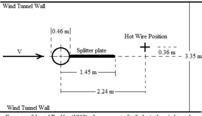
compress-ibility effects, the flow speed was limited to a Mach number of 0.25 or 85.07 m/s. The arrangement was shown in Figure 2.1.

Figure 2.1: Cylinder arrangement in the wind tunnel

Rahman et.al [14] found that, as Reynolds number becomes higher than 40 the flow reports a loss of symmetry in the wake. The studied also reported

the Strouhal number (St) is found to be 0.164 for Re=100.

Mittal and Kumar [2] reported the non-dimensional value of the vortex

shedding frequency is F_o = 0.234 for both cylinders while the non-dimensional

frequency corresponding to the cross-flow oscillations of both cylinders is 0.226.

Chandrakant and Swapnil [16] reported that the Strouhal number

in-creases with increase in Reynolds number and the number of vortices inin-creases

[image:20.595.119.508.259.483.2]

(21)

10

Ali and Edris [18] reported the computed drag coefficient (Cd) and the

Strouhal number in four numbers of nodes. For the number of nodes 28 000, 57 500, 82 500 and 103 000, the Cds were 1.345, 1.353, 1.366 and 1.366 while the

Strouhal numbers were 0.202, 0.204, 0.207 and 0.207.

Roshko [13] found out that vortex shedding was not observed at Re <

3.5x106. Below the value of Re < 3.5x106, no peak frequency occurred, but

above this value there appeared a strong spectral peak, said to be well above the

turbulence level.

Rahman et.al [14] observed that standard k-epsilon model computes drag

coefficients accurately. The realizable k-epsilon turbulence model is more

effec-tive for visualization of vortex shedding, while for the SST k-omega model, it is

recommended for high Reynolds numbers.

Mittal et.al [2] concluded that the oscillations of the cylinders result in an

alternate mode of vortex shedding and where the vibration of cylinders is usually

accompanied by an increase in drag.

Shao et.al [4] concluded that LES is capable of reproducing complex

subcritical turbulent wake behind a circular cylinder, but fine meshes and longer

time were required for the flow around the circular cylinder.

Bourguet et.al [6] concluded that the structural vibrations are mixtures

of standing and traveling wave patterns. A frequency ratio of approximately 2

can be established between the excited frequencies in the in-line and cross-flow

directions.

Mittal et.al [2] concluded that for a circular cylinder, flow separation

(22)

Chapter 3 Methodology

This chapter discussed about the methodology of this present work. This chapter

started with an introduction followed by physical model. In the physical model,

previous model has been chosen as a present model with some modification. The

numerical methods would discuss on discretization methods such as FVM, FEM

and FDM. This chapter also consists of the governing equation and the boundary

conditions of the present study based on previous study. In the CFD, it would

discuss on the process involved, such as preprocessing, solver and post-processing.

3.1 Numerical Study

This numerical study was carried out to investigate the effect of flow velocity on

the transverse vibration of bluff body in the CFD, together with the effects of

variation of the Reynolds number.

Obviously, the Reynolds number was an important non-dimensional

num-ber to determine the types of flow, either laminar or turbulent flow. Most flows

were turbulent in nature and it was applied in engineering too. Turbulence was

the chaotic nature of flow in motion showing random variation in space and

time.

Turbulence, contains eddies with different scales and sizes. These eddies

were always rotational in motion. Large scale eddies were responsible for the

carrying of energy and transfer of momentum in the flow. The large eddies,

extract energy from the mean flow and transfer it to the smallest eddies, where

(23)

12

energy was taken out of the flow through viscosity.

The well-known equations of fluid motion were known as the

Navier-Stokes equations. These equations have been derived based on the fundamental

governing equations of fluid dynamics. These fundamental was the continuity,

the momentum and the energy equations, which represent the conservation laws

of physics.

Continuity equation was based on the law of conservation of mass. Once

the concept applied to the fluid flow, the change of mass in a control volume was

equal to the mass that enters through its faces minus the total of mass leaving

its faces.

Momentum equation was expressed in terms of the pressure and viscous

stresses. Both pressure and viscous, stresses acting on a particle in the fluid. This would ensure that the rate of change of momentum of the fluid particles was

equal to the total of the force. This was due to the surface stresses and body

forces.

The energy equation was based on the First Law of Thermodynamics.

The rate of change of energy of a fluid particle was to be equal to the net rate

of work has done on that particle. This was due to surface forces, heat and body forces such as gravitational force. The energy equation describes the transport of

heat energy through a fluid and its effects.

A Navier-Stokes equation was a set of partial differential equations, with

the combination of all those fundamental principles which was the continuity,

mo-mentum and energy equations. Pressure and velocity of the fluid can be predicted

throughout the flow by solving these equations.

3.2 Physical Model

The physical modelled that used in this study was similar to the physical studied

by Rahman et.al [7]. A circular cylinder with diameter, d, was modelled in the

centre with a square flow domain is created surrounding the cylinder as shown in

Figure 3.1.

The computational domain for an upstream was 23 times of the circular

(24)

13

cylinder. The width of the domain was 50 times the radius of the circular cylinder

which was shown in Figure 3.1 together with the important dimensions [7].

Figure 3.1: Schematic diagram of the flow field around circular cylinder [7]

3.3 Numerical Methods

To solve the engineering problems, besides analytical and experimental methods,

the ability of numerical methods in fluid mechanics has increased. The used of

the numerical methods was to find numerical approximations to the solutions

where most of the differential equations could not be solved exactly.

In the Computational Fluid Dynamics (CFD), Navier-Stokes equations

were the basic governing equations. The equations were obtained by applying

Newton’s Law of Motion to a fluid element. It was also called as the momentum

equation, and supplemented by the mass conservation equation which was also

called the continuity equation and energy equation.

CFD was used to construct and discretise the governing equations, through discretisation methods such as Finite Difference Methods (FDM), Finite Element

[image:24.595.122.459.128.327.2]

(25)

14

3.3.1 Finite Volume Method

In a steady state solution the inlet and outlet mass flow rate would be obtained

equally. The change of momentum would equal the force exerted on solid

bound-aries. The solution of the steady state problems is performed by starting from

an arbitrary initial guess of the flow field and marching the equations forward in time until the flow becomes steady. If the flows entered and left every volume

were not equal, the conditions inside the volume must be changed and the flow

was not steady anymore.

Even the flow was at steady, the used in unsteady equations was found

to be very useful to solve the engineering problems. The FVM was based on

the discretisation of the Navier-Stokes equations. Every volume was contiguous with its adjacent volumes, and that the flow from recent volumes will enter the

adjacent volumes, and therefore, when a steady state reached, the flow was fully

utilized.

3.3.2 Finite Element Method

The Galerkin method was most commonly used formulation in FEM in fluid

me-chanics. The Galerkin method employs weighted residuals whereby their form

was usually assumed similar to the shape functions. The Galerkin method

ap-proximates the solution in terms of unknown nodal, and interpolated by the shape

functions.

3.3.3 Finite Difference Method

The conservation equations in differential form were approximated by replacing

the partial derivatives by approximations in terms of the nodal values of the

functions. Taylor series expansions or polynomial fitting were usually used to

obtain the derivatives of the functions with respect to the coordinates. This

yields an algebraic equation for each grid node in which values of neighbouring

nodes appear as unknowns. Although theoretically possible for unstructured

(26)

15

3.4 Governing Equations

The mathematical model of the finite volume method (FVM) that was used in

this study was similar to the model of numerical investigation of unsteady flow

passed a circular cylinder, studied by Rahman et.al [7]. The governing equations

for the unsteady flow of an incompressible viscous fluid passed a circular cylinder

were considered to the classical continuity and Navier-Stokes equations, which written in the following form:

div(~u) (3.1)

∂(u)

∂t +div(u~u) = 1

ρ

div(Γ∇u) (3.2)

On the left side of the equation (3.2) was the rate of change term and

the convective term and on the right side was the diffusion term, Ã= diffusion

coefficient which was used as the starting point in FVM.

ˆ

cv

∂(u) ∂t dv+

ˆ

cv

div(u~u)dv= 1

ρ

ˆ

cv

div(Γ∇u)dv (3.3)

In the second term of the left hand side of the equation (3.3) was the

convective term and on the right side was the diffusion term. By using the Gauss

divergence theorem, it could be rewritten as an integral over the entire boundary

surface of the control volume and the equation (3.3) became

∂ ∂t    ˆ cv (u)dv   + ˆ A

n.(u~u)dA = 1

ρ

ˆ

A

n.(Γ∇u)dA (3.4)

The rate of change term was equal to zero in the steady state case and

the equation (3.4) became

ˆ

A

n.(uU)dA= 1

ρ

ˆ

A

(27)

16

For the unsteady (time dependent) case it was necessary to integrate

with respect to time, t, over a small time interval, Δt i.e. from t to t + Δt,

Equation (3.5) became

ˆ ∆t ∂ ∂t    ˆ cv (u)dv   dt+

ˆ

∆t

ˆ

A

n.(u~u)dAdt= 1

ρ

ˆ

∆t

ˆ

A

n.(Γ∇u)dAdt (3.6)

In FVM, flow domain was divided into a number of control volumes or

cells which was called discretization. In order to solve the problem, equation (3.6)

needs to be discretized to be set up at a nodal point.

The resulting system of linear algebraic equations was then solved to

obtain the velocity and pressure distribution at each nodal point. Finally, the

drag and the lift coefficients were computed as follows:

CD =

D

0.5U_∞2d, CDP =

ˆ ₂π

0

Pwcos x dx, CDV =

2 Re

ˆ ₂π

0

ωwsin x dx (3.7)

CL=

D

0.5U_∞2d, CLP =

ˆ ₂π

0

Pwsin x dx, CLV =

2 Re

ˆ ₂π

0

ωwcos x dx (3.8)

Where, D and L represent the drag and lift force. The pressure coefficient

was defined as:

CP =

(P −P∞)

0.5ρU2d (3.9)

The subscripts P and V represent the pressure and viscous force. P_w is

the dimensionless wall pressure andωw is the dimensionless wall vorticity, defined

as

ωw =

ωR U∞

(28)

17

The dimensionless Reynolds number was given by:

Re= dU∞ρ

µ (3.11)

The Strouhal number was expressed as:

St= f D U∞

(3.12)

Where, the frequency of the vortex shedding, f (=1/T), the diameter of

the cylinder, d, and the free stream velocity, U∞.

The viscous forces of the turbulent flow were suggested to use standard

k-ε, realizable k-εand Shear-Stress Transport (SST) as suggested by Lakshmipathy

[7]. The standard k-ε model was based on model transport equations for the

turbulence kinetic energy (k) and its dissipation rate (ε) [7].

In the derivation of the k-ε model, it was assumed that the flow is fully

turbulent, and the effects of molecular viscosity are negligible. The standard k-ε

model is therefore valid only for fully turbulent flows [7]. The turbulent kinetic

energy, k, was given by:

k = 3

2(UavgI)

2 _(3.13)

Where, U_avg was the mean flow velocity and I was the turbulence

inten-sity. The turbulence intensity, I, was defined by:

I = 0.16(Re)18 (3.14)

The turbulence length could be written as l=0.07d and the turbulence

dissipation rate, ε, as,

ε=U 3 4

µ

k32

l (3.15)

(29)

18

which was approximately 0.09.

SST k-ε was another turbulent model, but modified to use with shear

stress turbulent [7]. The specific dissipation rate, ω, in the modify SST k-εcould

be found by,

ω = k 1 2

C 1 4

µl

(3.16)

3.5 Boundary Conditions

The uniform flow condition was imposed at the inlet boundary while pressure was

treated at the outlet boundary. The standard no-slip condition was used on the

surface of the cylinder, which was U_x = 0 and U_y = 0. At the top and bottom wall boundaries, the slip-flow condition was imposed where,

∂Ux

∂y = 0andUy = 0 (3.17)

3.6 Computational Fluid Dynamics

The investigation performed on the wake properties of the two dimensional flow

and a cylindrical bluff body by using the finite volume method. By using a

com-puter, the CFD solves the Navier-Stokes equations numerically for fluid flow.

Graphs and charts in CFD were used to analyze the flow characteristics in

order to compare with the previous researchers’ results. This study was performed in three steps, which were pre-processing, solver and post-processing by ANSYS

(30)

19

Figure 3.2: Steps Performed in CFD

3.6.1 Preprocessing

After creating a solid model of the domain, the first step of the CFD simulation

process was the pre-processing which will describe the geometry in detailed. The

domain of interest is then further divided into smaller segments which were known

as meshed.

The properties of the fluid acting on the domain need to be defined first before begin the analysis. These include external constraints or boundary

[image:30.595.122.358.85.442.2]

(31)

20

3.6.2 Solver

A solver calculates the solution of the CFD problem where the governing

equa-tions were solved. Identified physical problem such as fluid material properties,

flow physics model and boundary conditions were set to solve using a computer.

It was important to produce an accurate solution of the partial differential equa-tions by doing the convergence.

3.6.3 Post Processing

Flow phenomena would be presented in different methods, such as contour plots,

vector plot, streamlines, data curve and others related to the study. All those

methods would be used to analyze the results for appropriate graphical

repre-sentations to display the trends of velocity, pressure, kinetic energy and other

properties of the flow.

3.7 Methodology Summary

The methodology would be much better if it could be summarized. Therefore

a summarized methodology was clearly shown in a flowchart type as in Figure

(32)

21

[image:32.595.114.522.77.500.2]

(33)

Chapter 4 RESULTS AND DISCUSSION

This chapter discussed the extracted results of the cylindrical simulation. The

simulation was done in the flow of turbulence. The turbulence flow was ranged

from 70 000 < Re < 350 000. The results were analysed through the contours

and vectors of velocity and pressure coefficient figures. The Strouhal Number was

determined throughout the use of Strouhal figures, extracted from the analysis.

4.1 Validation

In order to validate, data’s from Simmons which was used by Roshko [13] had

been chosen. From the trend pattern, the extracted simulated data’s was then

satisfied as we could see as shown in the Figure 4.1.

(34)

23

Figure 4.1: Trending line validation between present study and Simmons

4.2 Velocity Magnitude

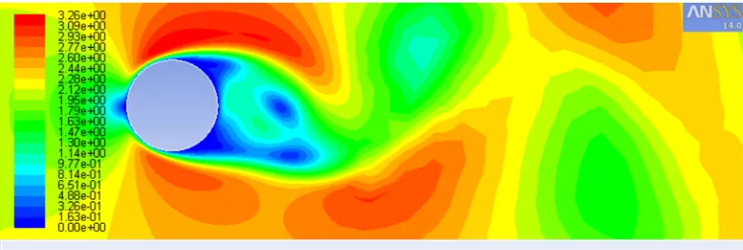
It could be seen as from Figure 4.2 to 4.13, the fluid flow after the boundary

layer at high Reynolds Number was an asymmetric flow. The vortex shedding is visualized throughout the contours and vectors of velocity magnitude.

As seen from the Figure 4.2 to 4.13, as the flow stream past the cylinder,

vortices were formed behind the cylinder. From all those figures, it could be seen,

as the flow speed increased, vortices were alternately shed on each side.

The vortex shedding clearly observed in all those figures and it could be

stated clearly that the vortex shedding proportional to the velocity magnitude

[image:34.595.118.478.65.290.2]

(35)

24

Figure 4.2: Contours of Velocity Magnitude at Re=70000

Figure 4.3: Vectors of Velocity Magnitude at Re=70000

[image:35.595.113.527.68.211.2] [image:35.595.114.525.285.430.2] [image:35.595.114.524.501.639.2]

(36)

Chapter 5 CONCLUSIONS AND RECOMMENDATIONS

From the research of simulation of Vortex Induced Vibration, the investigated

effect of flow velocity could be observed from the pressure coefficient and vorticity

magnitude.

It could be seen the increases of velocity which would also increase the

Reynolds number where the fluid flow past a bluff body creates vortices and were alternately shed on each side.

The vortex shedding frequencies were determined throughout the

ex-tracted results and data’s of the Strouhal number. It could be concluded, the

Strouhal numbers decreased with the increased of Reynolds number.

For the Reynolds number of 70 000 Re, 150 000 Re, 200 000 Re, 250 000

Re, 300 000 Re and 350 000 Re the Strouhal number were 0.017, 0.0194, 0.020,

0.0195, 0.0192 and 0.0184.

For the frequencies of vortex shedding, it could be concluded the

in-creased of Reynolds number would increase the frequencies while for the period

or duration of one cycle, decreased with the increased of Reynolds number.

For the Reynolds number of 70 000 Re, 150 000 Re, 200 000 Re, 250

000 Re, 300 000 Re and 350 000 Re the frequencies were 0.0174, 0.0425, 0.0584,

0.0712, 0.0841 and 0.094.

For the future work, there were still gaps that left behind in this research.

It could be recommended for the future research to study on different turbulence

model and different material.

(37)

References

[1] M. T. Asyikin, CFD Simulation of Vortex Induced Vibration of a Cylindri-cal Structure, Norwegian University of Science and Technology, Trondheim,

2012.

[2] S.Mittal and V.Kumar, Vortex Induced Vibrations of a Pair of Cylinders

at Reynolds Number 1000, International Journal of Computational Fluid

Dynamics, vol. 18(7), p. 601-614, 2004.

[3] X. Wang, B. Su and B. Su, Experimental study of vortex-induced vibrations

of a tethered cylinder, Journal of Fluids and Structures, vol. 34, pp. 51-57,

2012.

[4] J. Shao and C. Zhang, Large eddy simulations of the flow past two side-by-side circular cylinders, International Journal of Computational Fluid

Dy-namics, vol. 22(6), p. 393-404, 2008.

[5] H. Aref, M. Stremler and F. Ponta, Exotic vortex wakes—point vortex

solu-tions, Journal of Fluids and Structures, vol. 22, p. 929-940, 2006.

[6] R. Bourguet, G. E. Karniadakis and M. S. Triantafyllou, Lock-in of the

vortex-induced vibrations of a long tensioned beam in shear flow, Journal of

Fluids and Structures, vol. 27, pp. 838-847, 2011.

[7] Z. Pan, W. Cui and Q. Miao, Numerical simulation of vortex-induced

vibra-tion of a circular cylinder at low mass-damping using RANS code, Journal of Fluids and Structures, vol. 23, p. 23-37, 2007.

[8] S. Manzoor, J. Khawar and N. A. Sheikh, Vortex-Induced Vibrations of a

Square Cylinder with Damped Free-End Conditions, Advances in Mechanical

Engineering, vol. 5, 2013.

(38)

44

[9] F. Ponta and H. Aref, Numerical experiments on vortex shedding from an

oscillating cylinder, Journal of Fluids and Structures, vol. 22, p. 327-344, 2006.

[10] M. Dular and R. Bachert, The Issue of Strouhal Number Definition in

Cavi-tating Flow, Journal of Mechanical Engineering , vol. 55, pp. 666-674 , 2009.

[11] R. Gabbai and H. Benaroya, An overview of modeling and experiments of

vortex-induced vibration of circular cylinders, Journal of Sound and

Vibra-tion, vol. 282, p. 575-616, 2005.

[12] P. P. Patil and S. Tiwari, Numerical Investigation of Laminar Unsteady

Wakes Behind Two Inlinw Square Cylinders Confined in a Channel,

Engi-neering Applications of Computational Fluid Mechanics, vol. 3(3), p.

369-385, 2009.

[13] J. S. Leontini and M. C. Thompson, Active control of flow-induced

vibra-tion from bluff-body wakes: the response of an elastically-mounted

cylin-der to rotational forcing, in 18th Australasian Fluid Mechanics Conference,

Launceston, Australia, 2012.

[14] M. M. Rahman, M. M. Karim and M. A. Alim, Numerical Investigation of

Unsteady Flow Past a Circular Cylinder using 2-D Finite Volume Method,

Journal of Naval Architecture and Marine Engineering, vol. 4, p. 27-42, 2007.

[15] V. K. Patnana, R. P. Bharti and R. P. Chhabra, Two-dimensional unsteady

flow of power-law fluids over a cylinder, Chemical Engineering Science, vol. 64, pp. 2978-2999, 2009.

[16] C. D. Mhalungekar and Swapnil.P.Wadkar, CFD and Experimental

Analy-sis of Vortex Shedding behind D-shaped Cylinder, International Journal of

Innovative Research in Advanced Engineering, vol. 1(5), 2014.

[17] A. Kianifar and E. Y. Rad, Numerical Simulation of Unsteady Flow with

Vortex Shedding Around Circular Cylinder, in International Conference on

Theoretical and Applied Mechanics 2010; International Conference on Fluid

Mechanics and Heat & Mass Transfer 2010, Corfu Island, Greece, 2012.

(39)

45

[19] National Aeronautics and Space Administration (NASA), 12 Jun 2014.

[On-line]. Available: http://www.grc.nasa.gov/WWW/BGH/reynolds.html#.

[20] B. Sunden, “Thermopedia,” 16 March 2011. [Online]. Available:

http://www.thermopedia.com/content/1216/?tid=104&sn=1410. [Accessed

CFD simulation of vortex induced vibration of a bluff body structure by ANSYS fluent