3 dimensional simulation on drying of clay and alumina layers using computational fluid dynamics (cfd)

3 DIMENSIONAL SIMULATION ON DRYING OF CLAY AND ALUMINA LAYERS USING COMPUTATIONAL FLUID DYNAMICS (CFD)

SITI RAHAIDA BINTI ABDULLAH

A project report submitted in partial

fulfillment of the requirement for the award of the Degree of Master of Mechanical Engineering

Faculty of Mechanical and Manufacturing Engineering Universiti Tun Hussein Onn Malaysia

ABSTRACT

ABSTRAK

Computational Fluid Dynamics (CFD) telah digunakan untuk mensimulasikan aliran

CONTENTS

TITLE i

DECLARATION ii

DEDICATION iii

ACKNOWLEDGEMENT iv

ABSTRACT v

CONTENTS vii

LIST OF TABLE x

LIST OF FIGURES xi

LIST OF SYMBOLS AND ABBREVIATIONS xiv

LIST OF APPENDICES xvi

CHAPTER 1 INTRODUCTION

1.1 Background 1

1.2 Statement of Problem 3

1.3 Objective 3

1.4 Scope 3

CHAPTER 2 LITERATURE REVIEW

2.1 Introduction 5

2.2 Review of previous works on porous material 5

2.3 Computational Fluid Dynamics 18

2.4 GAMBIT 20

2.5 FLUENT Solver 21

2.6.1.2 Momentum Conservation Equation 25

2.6.1.3 Energy Equation 25

2.7 Open Close and Total Porosity 26

2.7.1 Pores Characteristic 27

2.7.2 Methods and techniques for production of 28 porous ceramics

2.7.3 Numerical Model Description 28

2.8 Pressure Drop 29

2.9 Flow in a structure Porous Media 30

2.10 Boundary Condition 31

2.10.1Inlet Boundary Condition 31

2.10.2Exit Boundary Condition 31

2.10.3Wall Boundary Condition 32

2.11 Convection Heat and Vapour Transfer Coefficients 32

2.12 Insulation of Drying 33

CHAPTER 3 METHODOLOGY

3.1 Introduction 35

3.2 Model Geometry Development Software 35

3.2.1 Discarded geometry and Mesh 36

3.2.2 Boundary Condition 42

3.3 Solution of Model 43

3.3.1 Fluent 6 Solver assumptions 44

CHAPTER 4 RESULT

4.1 Introduction 47

4.1.1 GAMBIT 47

4.1.2 Fluent 6 48

4.2 Case Study 1: Comparison of 2 dimensional with

2 porous media insulated and non-insulated 48 4.3 Case Study 2 : Comparison nodes of temperature

for 2 dimensional with 2 porous media 53

CHAPTER 5 CONCLUSION AND RECCOMENDATIONS

5.1 Conclusion 57

5.2 Limitation and Recommendation 58

REFERENCES 59

LIST OF TABLE

2.1 Material properties of SiC foam Modelled 8

2.2 Modelling Condition 10

2.3 Thermodynamic Properties of Ceramic Core 13

2.4 Transport Properties 15

2.5 Characterization of Alumina Powder 18

2.6 Solution Controls for FLUENT 22

2.7 Turbulence Models in FLUENT 23

2.8 Physical properties of material body for hygroscopic and

non-hygroscopic layer 29

3.1 Boundary conditions 42

LIST OF FIGURES

2.1 Coupled model flowchart 6

2.2 The velocity profile imposed at the inlet 7 2.3 Mass accumulation for various cases of air flow over gypsum 7

2.4 Mesh unit cell 9

2.5 Fluid and solid temperature distribution within the burner

Model for gas mixture 1 and 2 9

2.6 Schematic diagram of geometry used for the resin transfer moulding study.( The left side section of resin has been

truncated for clarity). 11

2.7 Schematic view of perform and inlet. The red subdomain represents the part of the geometry simulated by numerical

model. 12

2.8 Flow propagation of molten aluminium in porous perform 13 2.9 Contours of temperature distribution of air and exhaust flow 14 2.10 Contours of temperature distribution of ceramic core [unit:K] 14

2.11 Velocity contour in CASE 1 dryer 15

2.12 Velocity contour in CASE 2 dryer 16

2.13 Average moisture content curves at the top tray with 70°C

inlet air condition: CASE 1 and CASE 2 16

2.14 Average drying kinetic curves at the top tray with 70°C inlet

air condition: CASE 1 and CASE 2 17

2.15 Structure of open and closed pores 28

2.16 a) Velocity and temperature profiles for convective heat transfer b) Velocity and partial vapour pressure profiles for convective

vapour 33

2.17 Insulation diagram of drying chamber 34

3.2 2 Dimensional wireframe with three parts; inlet, porous media

and outlet 37

3.3 2 Dimensional wireframe with four parts: inlet, 2 porous media

and outlet 38

3.4 3 Dimensional wireframe with three parts: inlet, porous media

and outlet 39

3.5 3 Dimensional wireframe with four parts: inlet, 2 porous media

and outlet 39

3.6 2 Dimensional meshed model with 1 porous media 40 3.7 2 Dimensional meshed model with 2 porous media 41 3.8 3 Dimensional meshed model with 1 porous media 41 3.9 3 Dimensional meshed model with 2 porous media 42

3.10 2 Dimensional default solver options 44

3.11 3 Dimensional default solver options 45

4.1 2 Dimensional with 2 porous media static temperature plot versus flow time. (a) Insulated (b) Non-insulated 48 4.2 2 Dimensional with 2 porous media insulated (Contours of static

temperature 49

4.3 Contour 2 Dimensional with 2 porous media non-insulated

(Contours of static temperature) 50

4.4 2 Dimensional with 2 porous media pressure non-insulated

(Contours of velocity magnitude) 50

4.5 2 Dimensional with 2 porous media velocity magnitude plot

versus flow time (a) Insulated (b) Non-insulated 51 4.6 2 Dimensional with 2 porous media static pressure plot versus

flow time (a) Insulated (b) Non-insulated 52 4.7 2 Dimensional with 2 porous media mass flow rate plot versus

flow time (a) Insulated (b) Non-insulated 52 4.8 Node for 2 Dimensional with 2 porous media insulated 53 4.9 Node for 2 Dimensional with 2 porous media non-insulated 53 4.10 Temperature difference for the alumina insulating and

non-insulating 54

4.11 Temperature difference for the clay insulating and

4.12 3 Dimensional with 2 porous media velocity magnitude

contours 56

4.13 Sectional 3 Dimensional with 2 porous media velocity magnitude

LIST OF SYMBOLS AND ABBREVIATIONS

A,Ag,AU - Area ,area of gap, area of unit cell (m

2

)

α - Half yarn width (m)

B - Transducer for volumetric flow rate in permeability tester

Const - Constant in equation

Cp - Heat capacity (J/kg.K)

D - Mass diffusion coefficient [m2/s]

E - Young’s modulus (Pa)

→ - Force vector (N)

F - Frictional vector

G - Shear modulus (Pa)

g - Acceleration due to gravity (m/s2)

→ - Permeability tensor, effective permeability (m2)

m - Mass(kg)

P - Pressure (pa)

Q - Volumetric flow rate (m3/s)

Re - Reynolds number

r - Radial position (m)

T - Temperature (K)

t - Time (s)

V - Volume (m3)

V - Velocity (m/s)

→ - Velocity vector

Vf - Fibre volume fraction

W - Work done (W)

u - Superficial velocity (m/s)

GREEK SYMBOLS

, - Stress and Normal stress (N/m 2

)

- Non-Darcy coefficient in the Forchheimer equation

- Shear strain

- Micro element

- Fluid viscosity (kg/m.s)

- Fluid density (kg/m3)

- Yarn crimp angle ( ͦ )

∆∇

-Vector of operation

GLOSSARY

CFD - Computational fluid dynamics, using numerical methods to solve and analyze problem that involve fluid flows

Permeability - A measure of the ability of a porous material to transmit fluids

LIST OF APPENDICES

APPENDIX TITLE PAGE

A 3D drawing of the model with dimensions 61

B 2 Dimensional with 2 porous media residual 61

C 3 Dimensional with 2 porous media residuals 62 D 2 Dimensional with 2 porous media mass flow rate on outlet 62 E 3 Dimensional with 1 porous media residuals. 63

CHAPTER 1

INTRODUCTION

1.1 Background

Porous media have attracted in high diversions of the logical and mechanical gatherings amid the previous two decades. This is particularly valid for structuring methods that offer incredible adaptability and dependability. The efforts have been contributed on account of the fundamentally of porous materials as filters, dust collectors, absorbers, dielectric resonators, thermal insulation, bioreactors, hot gas collectors and automobile engine components. There could be named numerous different applications.

Davis (2010) in his research stated that more than 90% of alumina produced worldwide is utilized in production of Aluminium. This is because converting the naturally occurring bauxite into alumina is the necessary first step before it can be converted into Aluminium. The varied applications of alumina are due to its abundance and its multiple forms as well as its properties of stability, purity, refractoriness and chemical inertia. Due to their excellent mechanical properties, alumina based ceramic are being increasingly used as a substitute material for several application. These include the use of ceramic for abrasive and cutting tool.

the same size as a virus. Clays are very abundant at the earth’s surface; they form rocks known as shale’s and are a major component in nearly all sedimentary rocks. The small

size of particle and their unique crystal structures give clay materials special properties, including caution exchange capabilities, plastic behaviour when wet, catalytic abilities, swelling behaviour, and low permeability.

The attempt of alumina and clay in industry to achieve higher profitability, led to focusing on local raw material deposits and development of faster drying. The important of drying material towards alumina and clay measure structure are convection and conduction. Drying is mass transfer process resulting a removal of water or moisture from a solid, semi-solid or liquid (here after product) to end in a solid state. Transfer of internal moisture to the atmosphere and surface of the solid and its subsequent evaporation. It is an important process in the fine chemicals, food, pharmaceutical products industries, etc. Also, in some areas of synthetic chemistry, drying is a required process to obtain certain properties and characteristic. Convection heat and vapor transfer coefficients, also referred to as surface coefficient, are required to simulate the thermal performance of building envelope systems. Such theoretically depend on the following variables: velocity and type of air flow surface temperature, reference temperature of the air, surface relative humidity, reference relative humidity of the air and porosity at the surface of material.

The external flow analysis of porous body is important in drying thermal. Generally speaking, drying is a mass transfer process resulting can translate into significant design for the new model.

The modelling works were divided into two major parts. The first part deals with meshing the structured geometry complete with boundary layer. Second part was the simulation work at the different case study to measure the critical behaviour inside the porous body factors controlling transfer of heat from the surrounding to heated body to evaluate the velocity and temperature. Transfer of internal moisture to the atmosphere and surface of the solid and its subsequent evaporation.

provided the necessary data and knowledge leading to the establishment of alumina and clay membrane drying process which will be applicable to separation industry.

This section describes the background of study which consists of the explanation on software with previous data used to complete this project. This simulation work will allow the prediction complex behaviour of the dry process that lead to prediction of certain unmeasured variables. With this complete information on data on drying variables and its output, the complex drying of membrane structure can be established.

1.2 Statement of Problem

The determination of complex air flow behaviour through the material porous body is largely not yet implemented. Experimental or measurement work sometimes could not be established due to the complex small geometries in the material porous body design. In fact some crucial variables cannot be as certained via experimental work i.e diffusivity. With computational simulation and CFD modelling this problem can be resolved. In this work software do map or simulate the porous model. This method allows us to changes of any variables or parameter analysis at any time. With this technique, further investigation on system with different material mode of air flow and condition can be simulated and predicted.

1.3 Objective

The objective of the research is to determine the 2 layer porous media system that used the combination mechanism of porosity, permeability, density and related heat which enables an investigation of the influences for those certain process variable.

1.4 Scope

(ii) Study what are the processing parameters and the influenced of the variables in this flow technique.

CHAPTER 2

LITERATURE REVIEW

2.1 Introduction

The literature review was carried out to give detail background information of drying theory, phenomena and mechanism. Starting with review of previous works, it did give some idea and guideline to the direction of the research based on the current issues. It follows by literature works in related aspect i.e the material properties, density, porosity, permeability, heat capacity, heat conductivity and CFD method, etc, to gain and understand the drying process and fundamental.

2.2 Review of previous works on porous material

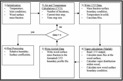
diffusion of moisture was solved with a control volume approach where relative humidity is the driving potential and variations of moisture content the desorption-sorption curve. This paper shows the flowchart for the solution process for the coupled heat and vapour transfer model. The data is transferred between each program using data files that are imported and overwritten within FLUENT and MATLAB.

Figure 2.1: Coupled model flowchart

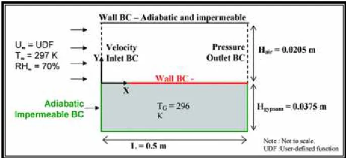
Figure 2.2: The velocity profile imposed at the inlet

Case 1 demonstrated the capability of the coupled model to calculate convective moisture transfer between air and gypsum panel for a number of air flow conditions. Next, a second case of vapour transport between air and porous material is presented to demonstrate that the coupled model can be used to calculate convective vapour transfer coefficients

Adam Neale et.al (2007) explained the result mass of moisture accumulated in the gypsum panels was calculated for four cases: one laminar case at 0.8m/s, 2.0m/s and 8.0m/s. Figure 2.3 demonstrates the sensitivity of the model to the regime of the air flow and the bulk speed of the air

Catharine Tierney et.al (2009) carried out computational fluid dynamics modeling of porous burners. This paper explains about system heat recirculation between the porous medium and the fuel stream leads to enhanced combustion behavior. In the research convective and radiative heat transfer models were added to the commercial CFD code ANSYS CFX, to describe the interaction between porous solid and the fluid.

Figure 2.4 provided the physical basis for the model. Accordingly, the one dimensional model consisted of a 240mm long domain. This entity was created as a ‘porousdomain’ and was therefore assumed to be homogenous porous body. Hamamre et. al (2007), Fend et. al (2005), Trimis et. al (2005) carried out the material properties of porous domain given in Table 2.1.

Table 2.1: Material properties of SiC foam modeled

Porosity (∅) 81%

Hydraulic diameter (dh) 0.83×10-3m

Area density (Ay) 500 m-1

Thermal conductivity (λs) 35 W m-1K-1

Heat capacity (Cps) 800 J kg-1K-1

Absorption coefficient (σa 46m -1

Scattering coefficient(σs) 224m-1

Figure 2.4: Mesh unit cell

The following boundary conditions were applied; i) gas inlet at the base of the domain, ii) gas outlet at the top surface of the domain and iii) symmetry boundaries on all other walls

In this work, no additional domain was included to consider the burner outlet surface. It may be necessary to include such a domain in future research to accurately model surface flames that can occur at very low concentration.

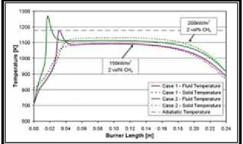
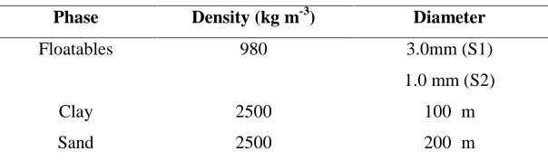
Figure 2.5: Fluid and solid temperature distribution within the burner model for gas mixture 1 and 2

K. Mohanarangam and D. W. Stephen (2009) carried out modelling a floating phase has been developed and tested on settling tank. The current model used for settling tanks is able to predict the settling of solids and the formation of a higher density layer of solids at the bottom of vessel. The simulations were performed by customizing the commercially available software ANSYS-CFX (release 10.0). Multiphase simulations were performed with clay, sand and a floating solid (density less than the continuous phase) as the secondary phase. The essentially sets up a volume fraction gradient of the floating phase. Two variants of particle sizes for the floating phase were used to access this phenomenon. Contour plots of the floating phase volume fraction are presented within the feed well as well in the cross-section of thank to depict the preferential concentrations of the phase.

Table 2.2 : Modelling condition Phase Density (kg m-3) Diameter

Floatables 980 3.0mm (S1)

1.0 mm (S2)

Clay 2500 100μm

Sand 2500 200μm

The phase considered in this study were sand, clay (both settling phase) and a floatable phase. The dispersed phase properties are summarised in Table 2.2. Two size variants of the floatables are used in the simulations to test their size dependency.

The time dependence of computed resin surface for this unsaturated porous medium exhibits good qualitative agreement with experimental results.

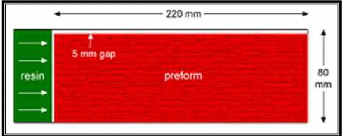
Figure 2.6: Schematic diagram of geometry used for the resin transfer moulding study. (The left side section of resin has been truncated for

clarity)

Young et.al (1997) explained the preliminary study of mould filling, including edge effects, has been undertaken. The geometry considered was similar to that described and consists of a rectangular channel with length of 220m and width 80mm (as shown in Figure 2.6). The preform comprised of an isotropic porous material, occupies the entire channel except for a 5mm gap at one side.

porosities in ASF and thereby optimizing the parameters involved in the infiltration process.

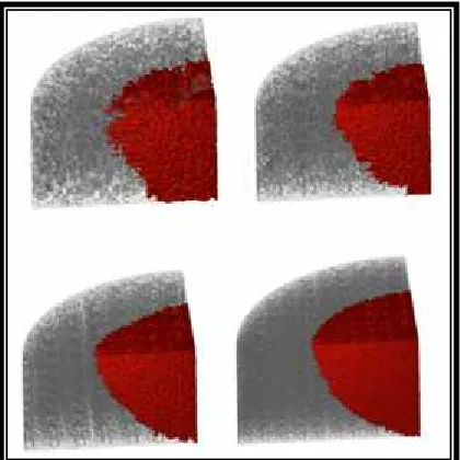
Figure 2.7: Schematic view of perform and inlet. The red sub domain represents the part of the geometry simulated by the numerical model.

Figure 2.8: Flow propagation of molten aluminium in porous perform

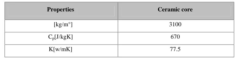
Young Hwan Yoon et.al (2009) conducted a theoretical analysis and CFD simulation on the ceramic monolith heat exchanger. In this paper explain about ceramic monolith heat exchanger is studied to find the performance of heat transfer and pressure drop by numerical computation and ξ-NTU method. The numerical computation was performed throughout the domain including fluid region in exhaust gas side rectangular duct, ceramic core and fluid region in air side rectangular duct with the air and exhaust in cross flow direction.

Table 2.3: Thermodynamic properties of ceramic core

Properties Ceramic core

Ρ[kg/m°] 3100

Cp[J/kgK] 670

K[w/mK] 77.5

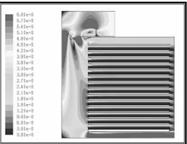
Figure 2.10: Contours of temperature distribution of ceramic core [unit:K]

Figure 2.10 shows the temperature profile of the ceramic core at the same condition on Figure 2.9. It can be also seen that the temperature is getting higher from left end to right end of the heat exchanger as the air temperature is increased from the left inlet to right exit.

Table 2.4: Transport properties

Property Value

H2O diffusivity in the dryer, 1.10 x 10-4m2/s

Air diffusivity in the dryer, 3.20 x 10-5m2/s

X diffusivity in the silica gel,Dm0 5.72 x 10-7m2/s

Density of silica gel,ρsg 1650kg/m3

Density of gas mixture,ρg 1.225 kg/m3

Viscosity of gas mixture,μg 1.7894 x 10-5kg/m.s

Figure 2.12 : Velocity contour in the CASE 2 dryer

Figure 2.14 : Average drying kinetic curves at the top tray with 70°C inlet air condition: CASE 1 and CASE 2

Chi-Young Jung et. al (2008) explained about the drying kinetics is evaluated with the change of solid moisture substances and temperature concerning time slipped by. The so-called drying curves, which describe moisture substance of silica gel particles with time, are indicated in Figure 2.13. As demonstrated, the moisture substance decrease linearly as time flows. Then the drying rate decreases, approaching the equilibrium moisture content in a form of parabolic curve. Figure 2.14 shows variety of drying rate consistent with time passed. At first, the drying rate constant increases linearly as time flows. In any case, around 60-80 minutes, linear lines turn into curves. With further elapsed time the rate gradually decreases with moisture content decrement.

with the porosity using semi empirical expressions of exponential type. The measured values for E modulus and Flexural strength are in good agreement with the calculated ones but the compressive strength deviated from predicted modeling behavior.

Table 2.5: Characterization of Alumina powder

Mean particle size, 0.22

Specific surface area,m2g-1 14.3

Density, (non fired), g cm-3 2.30

Fired density, at 1350°C, 1h,g cm-3 3.95

Dislocation density, cm-2 1012

Purity of Al2O3,% 99.99

Impurities, ppm Na (4), K(2), Fe(10), Ca(2), Mg(1), Si(12)

Vinod M. Janardhanan et.al (2011) conducted a computational fluid dynamics of catalytic reactors. In this paper, CFD simulation result have matured into powerful tool for understanding mass and heat transport in catalytic reactors. Initially, CFD calculation focused on a better understanding of mixing, mass transfer to enhance reaction rate, diffusion in porous media and heat transfer. The careful choice of the sub models (geometry, turbulence, diffusion, species and reactions involved, etc) and the physical parameters (inlet and boundary conditions, conductivity, permeability, viscosity, etc) is a precondition for reliable simulation results. Therefore, only the use of appropriate models and parameters, which describe all significant processes in the reactor, can lead to reliable results.

As explained earlier, these previous research, the critical parameter such as temperature, density, velocity and pressure are strongly influenced the drying process and the behaviour of alumina and clay properties.

2.3 Computational Fluid Dynamics

media geometries that will be discussed about in the ensuing chapters. Therefore, this requires a short foundation related to CFD. The physical features of any fluid flow are represented by the principal standards of mass, force and energy conservation. These standards can be communicated in term of non-linear partial differential equations.

CFD is an essential tool in fluid mechanics that approximates and numerically solves the fluid flow equation by discretising them over the domain of interest. Numerous modern applications, for example, petroleum reservoirs and heat exchangers involve fluid flow through channels and ducts with obstructions which take after porous media. Consequently we require CFD projects to model fluid flow through the channels and porous media to get a general understanding of the flow through these domains.

Additionally, in the process of designing systems, for example, cooling units, vehicles and plane, etc. different test with various parameters are obliged to acquire a general pattern for the reaction of the system. It is clearly unreasonable and tedious to manufacture these models and facilities to test them.

Advances of machine force have given a powerful method for assessing these models and acquiring answer for the issues within reach utilizing the CFD. Machine reproduction gives a general thought of the reaction of a system being outlined and lessens the quantity of trial tests that are needed for design purposes. Today, the utilization of CFD programming happens in displaying fluid flow issues because of its viability and efficient practicality.

Most fluid flow experienced in the mechanical applications are turbulent, in this manner a surmised and statically turbulence techniques are required. There are three principle methodologies to turbulent stream recreations in particular: (i) Direct Numerical Simulation (DNS), (ii) Large Eddy Simulation (LES) and (iii) Reynolds-Averaged Navier-Strokes (RANS)

In spite of the fact that CFD projects are advantageous to utilize, it is vital to comprehend and utilize the right models and arrangement calculations in the projects to acquire exact results without overabundance computational time. The recreations for this study will be run utilizing a CFD based programming bundle, FLUENT adaptation 6.3. The FLUENT programming bundle is arranged into two areas in particular: A matrix generator known as Geometry and Mesh Building Intelligent Toolkit "GAMBIT" and solver bundle "Familiar".

2.4 GAMBIT

A key venture in all CFD recreations is the development of the geometric model. The computational areas in this study will be made utilizing GAMBIT. GAMBIT is intended for developing the geometry and making a mixed bag of organized and unstructured frameworks to be utilized by the solver. GAMBIT gives a graphical client interface (GUI) to get inputs from the client.

The Gambit GUI utilizes fundamental steps for making the two and three dimensional geometries, meshing and assigning zone sorts to geometry. Different volumes, for example, 3D shape, cylinders, cones and pyramids are likewise accessible. The complex three-dimensional models are made utilizing these volumes. The contiguous volumes and countenances can be united, subtracted and met with one another. For a top to bottom talk in regards to the utilization of every particular order in GAMBIT, the reader is referred to Fluent Inc. (2005).

For any given domain, GAMBIT recognizes the outer sides of the geometry as walls and the space between these sides as interior which can either be a fluid or solid. So it is important that after geometry and mesh generation, the boundary conditions should be specified according to the model specifications. The zones should also be set as either a fluid or solid. After the above summarized steps are completed, from the file menu in GAMBIT the mesh file is exported to FLUENT.

2.5 FLUENT Solver

After the mesh file has been exported to FLUENT, several user controlled options must be specified in the solver. The FLUENT solver supplies various options, of which only few relevant to this work will be mentioned. Once the mesh file is opened in FLUENT , it checks the grids and if there are no errors occurs, then the parameters can be st to solve a particular problem.

The FLUENT solver uses a finite-volume procedure, which converts the governing differential equations presented in Mathematical model into algebraic form, together with the SIMPLE (Semi-Implicit-Method for Pressure Linked Equations) algorithm to solve these equation numerically, Fluent Inc. (2005). For the discretization of equations the second-order upwind scheme was selected for all the laminar flow simulations carried out. Details about the numerical methods in general and other discretization schemes can be found in literature, by Patankar (1980).

The FLUENT solver utilizes a finite-volume methodology, which changes over the representing differential equations exhibited in Mathematical model into mathematical structure, together with the SIMPLE (Semi-Implicit-Method for Pressure Linked Equations) algorithm to understand these equation numerically, Fluent Inc. (2005). For the discretization of mathematical statements the second-order upwind plan was chosen for all the laminar flow simulations carried out. Insights about the numerical methods in general and other discretization plans can be found in literature, by Patankar (1980).

two types of solvers: coupled and segregated and the latter will be used in all the simulation conducted in this work. The default solution methods defined in FLUENT are, 2D space, segregated solver, implicit formulation, steady flow and absolute velocity formulation. The segregated approach solves the governing equation sequentially using the iterative method while, with the coupled solver, the equation are solved simultaneously.

Definition of the physical properties of the fluid and boundary conditions as specified in GAMBIT, is also a requirement for setting up the numerical model. For fluid material, the values of the following parameters are required: density, viscosity, thermal conductivity and specific heat capacity. The mass flow rate or pressure gradient should be specified in the case of the periodic boundary condition.

The velocity boundary condition is used to define the flow velocity at the flow inlets and the pressure outlet boundary condition requires the specification of gauge pressure at the outlet. In case of asymmetric physical geometry, a symmetric boundary condition is used this sets the normal velocity gradient to zero. The outer boundaries defined as walls, mean that the flow does not exist at these boundaries, and the boundary condition at these walls is presented by no slip condition.

Selection of proper numerical control, for updating the computed variables after each iteration, and modelling techniques is of importance to speed up convergence and stability of the calculation. The default under-relaxation factors shown in Table 2.6 were used to perform the laminar flows calculations. Since numerical computations can only give approximated values, a check for the convergence of the equations is made. Convergence in FLUENT is obtained by monitoring the scaled residuals and flow parameters at critical points as well as successively reducing the value of criterion.

Table 2.6: Solution Controls for FLUENT

Under Relaxation Discretization Converge Criteria

Pressure 0.3 Pressure Standard Momentum 0.001

Density 1.0 P-V-C SIMPLE X-Velocity 0.001

Table 2.6 (continued)

Under Relaxation Discretization Converge Criteria

Momentum 0.7 Momentum ( − ) 1st–O-U

Momentum (RSM) ₁st_–O-U

T-k-E ( − & RSM) ₁st_–O-U

T-D-R ( − & RSM) ₁st_–O-U

FLUENT also provides a variety of turbulence scales and prediction methods. As mentioned previously, the two approaches for the turbulence modelling that FLUENT offers are RANS and LES. In this study two RANS equations models, namely: the Standard − model and the Reynolds-Stress model will be used to model the fluid flow through the timber stack ends at high Reynolds numbers. Various RANS equation models are tabulated in Table 2.7 and various techniques are generally described in Fluent Inc. (2005)

Table 2.7 : Turbulence Models in FLUENT

Model Descriptions

Spalart Allmaras One-Equation RANS based model

Standard − Two–Equation RANS based model

RNG − Two–Equation RANS based model

Realizable − Two–Equation RANS based model

Standard − Two–Equation RANS based model

Shear-stress transport (SST) − Two–Equation RANS based model

Reynolds-Stress model (RSM) Two–Equation RANS based model

Large eddy simulation LES model

repeat of the numerical simulation. If the solution does not change, grid independence results are obtained otherwise, the process of refining the grids continues.

2.6 Computational Fluid Dynamics Model Equations

In this study the single phase model was used for solving the respective category problems. This model will calculate one transport equation for the momentum and one for continuity for each phase, and then energy equations are solved to study the thermal behaviour of the system. The theory for this model is taken from the ANSYS FLUENT 6.3.

2.6.1 Single Phase Modelling Equations

The single phase model equations include the equation of continuity, momentum equation and energy equation (ANSYS Fluent 6.3). The continuity and momentum equations are used to calculate velocity vector. The energy equation is used to calculate temperature distribution and wall heat transfer coefficient. The equation for conservation of mass, or continuity equation, can be written as follows:

2.6.1.1 Mass Conservation Equation

The equation for conservation of mass, or continuity equation, can be written as follows:

+ ∇. ( →) = (2.1)

REFERENCES

Adam Neale et.al (2007) “Coupled Simulation of Vapor Flow between air and a Porous

Material” ASHRAE

Ashish Kumar Pandey et.al “A computational Fluid Dynamics Study of Fluid Flow and

Heat Transfer in Micro channel” Master of Technology in Chemical Engineering. A. Hussain et.al (2006) “ Heat and mass transfer in tubular ceramic membranes for

membrane reactors”.

Amar Al-Fathah Ahmad (2009) “CFD Simulation of Temperature Distribution and Heat Transfer pattern Inside C492 Combustion Furnace”.

Carl Persson(2012) “CFD Simulation and Validation of Downdraft Pottery Furnace”. Catharine Tierney et.al(Dec 2009) “Computational Fluid Dynamic Modelling of Porous

Burners”

Chi Young Jung et.al (2008) “Two-dimensional simulation of silica gel drying using computational fluid dynamics”

D. Segal(1989) “Chemical synthesis of advanced ceramic material”, Cambridge

University Press

D.M Liu, V Dixit(1997) “Porous materials for tissue engineering Uetikon”- Zurich, Trans Tech Publications,

D.M. Liu (1996)“Porous Ceramic Materials: Fabrication, Characterization, Applications, Aedermannsdorf, Trans. Tech” Publ.

Hannah Duscha et.al (2012) “Computational Fluid Dynamics Analysis of Two-Phase Flow in a Packed Bed Raector” Degree of Bachelor of Science in Chemical

Engineering

H. N Suresh et.al (1999) “ Drying of Porous Material using Finite Element Method)”.

J.S. Magdeski (2010) “The Porosit Dependence of Mechanical Properties of Sintered

Karen davis (2010) “Material review: Alumina (Al2O3)” Student PhD in Chemical Engineering at School of Doctoral Studies.

K.Mohanarangam and D.W.Stephen(Dec 2009) “CFD Modelling of Floating and

Settling Phase in Settling Tanks”

K. Sommer(2004) “Size Enlargment Ullmann’s Encyclopedia of Industrial Chemistery,

M.W.Barsuom. (2003)“Fundamental of ceramics” MPG Books Ltd Bodmin, Cornwall, IOP Publishing Ltd

Mark.L et.al(1999) “Modelling of Flow in Porous Media and Resin Transfer Moulding

Using Smoothed Particle Hydrodynamic”,

Ravaglioli, A. Krajewski(1997) “Implantable Porous Bioceramics in Porous Material for Tissue Engineering ed. D.M Liu and V. Dixit. Trans Tech Publication Switzerland

Sam E.H Robjer Gullman (2010) “ Development of evaporation models for CFD”

S R Tennison (1996) “Microporous Ceramic Membranes For Gas Separation Processes”

Sapto W.W et.al “CFD Simulation For Dryer Optimization” Universiti Teknikal

Malaysia Melaka.

S. Turek et.al (2009) “On special CFD techniques for the efficient solution of dynamic porous media problems”,

Shizhao Li et.al (2010)“A CFD Approach for Prediction of Unintended Porosities in Aluminium Syntactic Foam: A Preliminary Study”

Vinod M. Janardhanan et.al(2011) “Computational Fluid Dynamic of Catalytic

Reactors” Version 25.03.2011

Xueling Xiao (August 2012)“Modelling the structure –Permeability Relationship for woven Fabrics”

Young Hwan Yoon et.al (August 2009)“A Theoritical Analysis and CFD Simulation on