Small Electrical Loop Analytical Calculation

Small Electrical Loop Analytical Calculation

René Harťanský

1, *

_{, Peter Mikuš}

1,

_{, Lukáš Maršalka}

1

_{, Jozef Slížik}

1

_{, Ladislav Matejička}

2

1_{Institute of electrical engineering, Faculty of Electrical Engineering and Information Technology, Slovak University of Technology in}

Bratislava, Bratislava, Slovakia

2_{Trenčín University of Alexander Dubček, Trenčín, Slovakia}

*Corresponding Author: [email protected]

Copyright © 2013 Horizon Research Publishing All rights reserved.

Abstract

The article deals with vector potential calculation of the small electrical loop. The method of integral analytical expression solves the problem in the details. This type of integral is the same as in the theory of antenna. This method is simpler than standard method and it makes some connection between radiation theories of point source at the far field and loop at the near field.

Keywords Small Electrical Loop, Far Field, Near Field,

Antenna, Integral Analytical Expression, Vector Potential

1. Introduction

In the theory of antenna is often needed to express an electric or magnetic field in scattering area via wave equations. Possibilities of realization of this problem was well-established by using the vector potential. This vector potential significantly simplified the solution of the wave equations.For the acquisition of the vector potential is needed the following mathematical form:

dV R e z y x J A

V

jkR ∫∫∫

= ( `, `, `) − 4π

µ

(1)

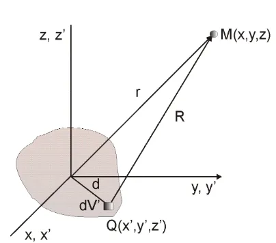
where R is dimension of displacement vector from radiation place to observation place as it is shown in figure1. Inthe figure is possible to define R which is dependent from displacement of observation point in centre of coordinate system and along to emitter shape.

2 2

2 _{( `) ( `)}

`)

(x x y y z z

R= − + − + − (2)

[image:1.595.329.531.238.416.2]

The equation (1) solve the most complicated geometry of emitter in a difficult way. And therefore in literature are only approximation solutions for example [1] and this type of solution is wastingit´s universality.The goal of this paper is to find an accurate solution of vector potential for the concrete emitter type. The name for this emitter is the small electrical loop.

Figure 1. Determination of displacement from observation point

2. Small Electrical Loop Antenna

Dimension of this antenna type are smaller than the smallest wave length in which the antenna is located. According to [2] the current distribution along loop is constant:

const.

`

I

_Φ

=

(3)

It means that solution must be concentrate to the integral solution.

( )

( )

jkR b

e

_dV

R b

V

−

∫∫∫

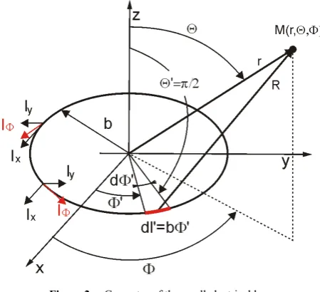
(4)

This is directly tied with loop antenna geometry. For example, the classical solution can be explained now. On the base of loop antenna geometry (see figure 2) can be explained the dimension of position of vector R(b).

2

2

( )

2 sin cos `

R b

=

r

+

b

−

br

Θ

Φ

(5) Then there is obtained the following function under the integral

2 2 2 sin cos `

( )

2

_{2 2 sin cos `}

jk r b

br

e

f b

r

b

br

−

+ −

Θ

Φ

=

[image:2.595.304.556.73.390.2]

In the literature the integration of this function is solved with approximation of suitable series. It´s form is simplifying by that. Literature [1] describes the evolution of function to Mac-Lauren series in point b=0. In a real case b is not equal to zero. This approximation is valid only for a big distance of r. In this case the loop appears as infinitely small.

Figure 2. Geometry of the small electrical loop

In this case can be seen the loosing of solution objectivity and expression of function g(b) is unnecessarily demanding.

0 b r

if →∞ then → (7)

In this modification the solution is not usedin the approximation of relation (6) but in the approximation of function R(b) and_e−jkR(b)_{.Each of these functions is estimated} in point afield 0. While multiplication of estimations can obtain complete approximation.

) ( ) ( ) ( 1 )

( ( ) _{hb g b}

b R e

b

f ₌ −jkRb _{⋅ = ⋅ (8)}

According to Taylor sentence is valid:

2 ) (' ' ) (' ) 0 ( )

( 0 2

b g b b g g b

g = + b= + ξ (9)

whereξ is point from interval (0,b). Function g(b) can be formulated from following expression.

b b g g b

g( )= (0)+ (' )b=0 (10) and the approximation fault is

b b

g

b =

ξ

≤

ξ

≤

ε

0 2 ) (' ' ) ( 2

1 (11)

denote ) ( 1 ) ( b R b

g = (12)

and calculate the derivation of displacement vector. The result of calculation was used in expression of Taylor series.

) ( ) (' ) (' ₂ b R b R b

g =− (13)

from this

(

sin cos `

)

( ) 1 1 ) ( 1 1

2b b

r r b

R = − Θ Φ +

ε

(14)

where ε1(b) is approximation fault and her valuation is

) ( ) ( ' 2 ) ( ) (' ' ) ( ) ( ' ) ( 2 ) ( ) (' ' ) (' ' 3 2 2 4 2 2 b R b R b R b R b R b R b R b R b R b g + − = = + − = (15) next ) ( ` cos sin ) (' b R r b b

R = − Θ Φ (16)

after modification

(

)

) ( ` cos sin ) ( 1 ) ('

' ₃ 2

b R r b b R b

R = − − Θ Φ (17)

from this

(

)

(

)

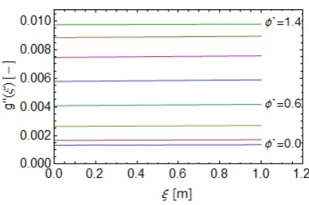
) ( ` cos sin 2 ) ( ` cos sin ) ( 1 ) ( 1 ) (' ' 5 2 5 2 3 '' b R r b b R r b b R b R b g Φ Θ − + Φ Θ − + − =       = (18)

To determine the error of approximation we must know the course of the function g’’(ξ), where 0≤ξ≤b.Mathematical determination of the functioncourse is the demanding and so it´s course can be expressed by using multiple graphs.

[image:2.595.64.289.156.361.2]

Figure 3. Graph of functiong’’(ξ) for r>>b aΘ=0.2

[image:2.595.306.541.438.742.2]

[image:3.595.68.286.70.214.2]

Figure 5. Graph of functiong’’(ξ) for r>>b aΘ=1.2

Figures 3-5 show that the value of the second derivation depends on anglesΘ a Φ`, but the function is almost constant when it depends on radius b. And so, for the setting of the estimation error of the functiong(ξ)we can write:

0 * * 0

) 0 (' ' ) ('

'

ξ

= g ≤

ξ

≤

ξ

ξ

>

g  (19)

If R(b)>>b then R(b)

→

r and

3 2 2 _{cos `}

sin 3 1 ) 0 (' '

r

g = − + Θ Φ (20)

After this can be obtained the approximation fault

2 ` cos sin 3 1 )

( 3 2

2 2

1

b r

b → − + Θ Φ

ε (21)

If behind g(b) choose following expression now

( )

( )

jkR b

h b e

=

−

(22)

and use Taylor series, we obtained this

(

)

'

( ) (0) ( )

( ) ₂( )

0

jkR b jkR jkR b

h b e e e b b

b

ε

− − −

= = + +

=

(23) where

(

_{( )}

)

''

2

( )

0

2

b

e

jkR

ξ

b

₂

b

ε

=

−

≤ ≤

ξ

(24)

Similarly as in the appointment case, there can be calculated the relevant derivations.

(

( )

)

'

( )

(

'( )

)

sin `cos

( )

( )

jkR b

jkR b

e

e

jkR b

b r

jkR b

jke

R b

−

₌

−

₋

₌

−

Θ

Φ

−

= −

(25)

and

(

_e−jkR(0)

)

'_{= jke}−jkrsin_Θcos_Φ`₍₂₆₎ By substituting (26) into (23), the approximation of the exponential function:

( )

_{sin cos}

₂

_{( )}

jkR b

jkr

jkr

e

−

=

e

−

+

jkbe

−

Θ

Φ +

ε

b

(27)

Approximation fault ε2(b) is calculated in the same manner

as in the previous case

(

)

{

(

(

(

( )

)))}

`sin cos

) ( 2 `sin cos

) ( )

( ''

) ('

' 2 2

3 ) ( )

(

b kR j r

b bkR r

b kR b jr k b R e e

b

h jkRb jkRb

+ − Θ Φ

+ −

Θ Φ +

+ −

=

= − −

(28)

Similar to previous case, for the setting of the approximation error we must know the course of the function h’’(ξ), where 0≤ξ≤b. It can be done in the graph:

Figure 6. Graph of the functionh’’(ξ) for r>>b aΘ=0.2 in Fraunhofer zone

[image:3.595.286.530.196.679.2]

Figure 7. Graph of the functionh’’(ξ) for r>>b aΘ=0.6 in Fraunhofer zone

Figure 8. Graph of the functionh’’(ξ) for r>>b aΘ=1.2 in Fraunhofer zone

0 * * 0 ) 0 (' ' ) ('

'

ξ

≤ h ≤

ξ

≤

ξ

ξ

>

h (29)

If R(b)>>b then R(b)

→

r and

(

)

(

sin cos `

)

) 0 (' '

2

2_{Θ Φ}

+ − + ⋅ − = − kr j j k r e

h jkr ₍₃₀₎

After this can be obtained the approximation fault

(

)

(

sin cos `

)

₂

)

( 2 2 2

2 b e_r k j j kr b

jkr Φ Θ + − + − → −

ε (31)

Here was created the space for integrand calculation in distribution of vector integral, which (without current distribution) have acquired form

(

)

(

)

) ( ` cos sin 1 ` cos sin 1 ) ( ` cos sin 1 ) ( ` cos sin ) ( 1 ) ( ) ( ) ( 2 2 2 1 2 2 b b r jk r jkb r e b r b r b jkbe e b R b jkR e b g b h jkr jkr jkr ε ε ε +       Φ Θ       ₊ + Φ Θ + ⋅ =     

 _{+ Θ Φ +}

⋅ + Φ Θ + = − = ⋅ − − − (32)

whereε(b) is approximation failure of the integrand an after simplification has the following form:

) 0 ( ) 0 ( 1 ) 0 ( ) 0 ( ) ( 2 1

1 ε ε

ε ε ε       + + = ≤ − r e

b jkr ₍₃₃₎

3. Vector Potential of the Small

Electrical Loop

In this paper was prepared the mathematical apparatus for vector potential calculation of the small electrical loop. For the next calculations there are needed the current formulation which are flowing across the loop. Since the loop is electrically small and there is not assumption of still wave on loop for this case the current flowing cross loop is constant IΦ

= const. and the current has everywhere the same amplitude

and phase.

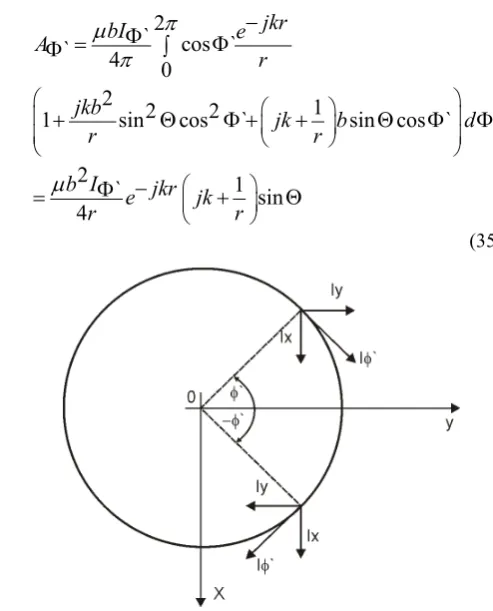
For the calculation there must be chosen two elements on loop. Their localization is symmetric because of y axis. In this elected elements will be constant current (can be considered on behalf of elementary emitters) but the orientation in space is changed. In figure 3 can be seen the current IΦ which is possible resolved on two components Ix

and Iy. Components Ix are affecting in the same orientation

and are added. The components in Iy direction are affecting

in mutually opposite orientation and their effect is eliminated. The result of this consideration is: the field in radiation zone is created only from Ix component. This current is possible

expressed with aid of following relation.

` cos

` Φ

=I_Φ

Ix (34)

Put equation (34) into the integral of vector potential and obtained result is

2

`

_{cos `}

`

₄

0

2

₂

₂

₁

1

sin

cos

`

sin cos `

`

2

_`

₁

sin

4

jkr

bI

e

A

r

jkb

_jk

_b

_d

r

r

b I

_e

_jkr

_jk

r

r

π

µ

π

µ

 _{ }   _{ }   _{ }         

−

Φ

=

_∫

Φ

Φ

+

Θ

Φ +

+

Θ

Φ

Φ

−

Φ

=

+

Θ

[image:4.595.301.548.130.436.2]

(35)

Figure 9. Determination of electrical current across small loop

4. Discussion

To have an idea about the adequacy of the used approximation it is necessary to give some examples of the approximation failure. These errors arose by simplifying the calculation of Taylor series. In the calculation of the vector potential we are primarily interested in errors depending on the radius of the loop antenna and errors depending on the observation angle θ; for the expression will be used so called relative error.

[

]

% 100 ) ( ) ( ) ( ) ( ) ( ) ( ) ( ) ( % 100 ⋅ + ⋅ + ⋅ − ⋅ = ⋅ − = b b g b h b b g b h b g b h func real func real func approx ε ε δ (36)

[image:5.595.84.269.86.215.2]

Figure 10. Approximation relative error depended on loop perimeter

Figure 11 showsagain the dependence of the relative error of approximation of the integrand in (4) on the radius loop. In this case, however, it is at a distance of k.r = 100. We can see that in the10-fold increase of the distance r, the approximation error stays nearly the same as in the previous case.

Figure 11. Approximation of relative error depended on loop perimeter

It shows a good approximation of the integrand in (4) for Fraunhofer zone.

In both cases (figure 4 and figure 5), the calculation of the relative error is made for such an arrangement of the observation point, where we expect the greatest radiation of the loop.

Figure 12. Approximation relative error depended on θ angle

Figure12 shows the dependence of the relative error of approximation of the integrand of equation (4) depending on change of the angle of observationθ. The dependence was calculated for Fraundhofer zone k.r = 10. We can see that the

approximation has the biggest differences from the actual function at angleπ/2 rad. In this case it is not a fatal error because the error is very small and it influencesshape of radiation pattern only in the direction of the maximum radiation.

In figure 13 is shown the same situation as in figure12 with the difference that the radius of the loop increases on b = 0.1 λ.

Figure 13. Approximation relative error depended on θ angle

We can see that there was increase of the relative error. In contrast to previous cases, this increase is significant.

5. Conclusion

In this paper is presented the alternative possibilities of vector potential solution for electrically small loop antenna. In comparison with classical solution where is integrand of vector potential developed to Mac-Lauren series and approximation is sufficiently exact only for loop whose dimension are very close to zero. In this case the information about field shape in fare zone is losing at calculation. The loop is no appearing in this far zone as infinitesimally small. Approximation which was used in our solution is significantly exact for real loop dimension. The reinstate approximation into the integral of vector potential is obtained relation (35) which has the same expression as is asserted in literature [1]. There is not an expression of the approximation error of integrand (4)in literature [1]. Thanks the expression of the approximation error of integrand (4)we get the following conclusions:

●the approximation error is negligible in the far field in the case that the radius of the loop is b<0.01 λ;

● the approximation error is significant in the direction of the radiation θ=π/2. This fact can influence the gain of loop antenna and radiation pattern of loop antenna or loop antennas array.

Acknowledgement

[image:5.595.330.534.178.315.2] [image:5.595.88.264.321.442.2] [image:5.595.74.284.546.682.2]

technology in rubber industry and by the project VEGA 1/0963/12 - Validation methods of selected test of EMC.

REFERENCES

[1] Balanis, A., C.: Anthenna Theory Analysis and Design, Haper& Row, Publishers, New York, 1982

[2] Vavra, Š., Turán, J.: Antény a šírenieelektromagnetickýchvĺn, Alfa, Bratislava, 1989

[3] Jarník, V.: Diferenciálnípočet I, Academia, Praha 1974 [4] Bittera, M., Kamenský, M., Smieško, V.: Broadband