Electromagnetic Force Calculation Method in Finite Element Analysis for Programmers

Electromagnetic Force Calculation Method in Finite

Element Analysis for Programmers

Young Sun Kim

Department of Electrical and Electronic Engineering, Joongbu University, Goyang, South Korea

Copyright©2019 by authors, all rights reserved. Authors agree that this article remains permanently open access under the terms of the Creative Commons Attribution License 4.0 International License

Abstract

Background/Objectives: Finite element method has been used widely for structural analysis of electromagnetic systems for a long time. Maxwell stress sensor and principle of virtual work are used to calculate electromagnetic force from finite element analysis results.

Methods/Statistical analysis: In this paper, specific methodologies were presented when programming was coded directly without the use of commercial software. Maxwell stress sensor is the amount of tension expressed by the interaction of electromagnetic force with mechanical physical quantity. Findings: When calculating the electromagnetic force, a method of integration was proposed when trying to integrate by selecting the element around the body to obtain the force. Also, the principle of virtual work is to induce electromagnetic force from the derivation of system energy. This method was proposed to differentiate the matrix in the finite element method.

Improvements/Applications: We selected a 3-dimensional Axisymmetric model to validate the usefulness of the proposed method of calculation.

Keywords

Electromagnetic Force, Finite Element Method, Maxwell Stress Tensor, Principle of Virtual Work, System Energy

1. Introduction

The finite element method(FEM) is one of the numerical analysis techniques that divides a continuum structure into finite number of elements and then performs calculations based on an approximate solution based on the energy principle for each domain. A finite number of elements use elements of a one-dimensional straight line, a two-dimensional triangle, a square, and a three-dimensional tetrahedron [1]. CAE is the method most commonly used for structural analysis and electromagnetic field analysis. It is a method developed for stresses and electromagnetic field analysis of complex shapes. This

technique requires a high-performance computer because it performs extensive system matrix calculations, but it can also be used as a personal computer due to recent computer developments. Other numerical methods include finite difference method and boundary element method [2, 3].

In electromagnetics, the Maxwell stress tensor is a 3 × 3 tensor that represents the strain generated by the electromagnetic field. The Maxwell stress tensor is a symmetrical 2-order tensor used in classical electromagnetics to represent the interaction between electromagnetic force and mechanical momentum. Calculation of the force exerted by a conductor carrying a currents in an uniform magnetic field is easily accomplished by Lorentz's law of force [4]. However, when calculating the magnetic force received by a ferromagnetic body in a magnetic field, the current term in the Lorentz equation must be replaced by a magnetic field or magnetic flux density. At this time, when the formula is developed by using the Maxwell stress tensor, the electromagnetic force can be easily expressed [5-7].

The concept of virtual displacement in relation to the concept of virtual operations in analytical mechanics is meaningful only when discussing motion-constrained physical systems. In the special case of infinite displacement, the virtual displacement means a minute change in the position coordinates of the system so that the constraint is satisfied [8-10].

2. Mathematical Theory for

Electromagnetic Force

The basic principles of the Maxwell stress method and the virtual displacement method, which have been used for the calculation of the electromagnetic force, are explained by using the results of the finite element analysis. First, a mathematical process for deriving the Maxwell stress from the Lorentz force is described. The magnetic force density is expressed by the current density and the magnetic flux density as follows.

]

/

[

N

m

3

B

J

f



=



×



(1) The current density term by Ampere's law are as follows.

)

(

1

0

B

J



=

∇

×



µ

(2)

B

B

f







×

×

∇

=

1

(

)

0

µ

(3)

Therefore, the force exerted by a magnetic field on an object having a volume V is as follows.

∫

=

v

f

dv

F





(4)

Using the vector identity, the magnetic flux density curl operation is developed as follows.

2

2

1

)

(

)

(

∇

×

B



×

B



=

B



⋅

∇

B



−

∇

B

(5)

Therefore, the force of the volume is given by the following equation.

[

_∫

⋅

∇

−

_∫

]

=

v

B

B

dv

s

B

n

ds

F

1

(

)

2

ˆ

0







µ

(6)

Where

s

is the surface of volume

_V

and

_n

ˆ

is the extrinsic unit vector perpendicular to

s

.

∫

⋅

∇

=

∫

⋅

v

(

B

)

B

dv

s

B

(

B

n

ˆ

)

ds









(7) When the extrinsic unit vector and divergence theorem are applied, the electromagnetic force equation can be expressed as Maxwell stress as follows.

∫

∫

⋅

=

⋅

=

s

v

f

d

v

d

s

F







P



(8) The following is a concrete expression of Maxwell's stress and a representation of a unit vector.

n

B

B

B

n

ˆ

2

1

)

ˆ

(

1

₂

0

0

µ

µ

⋅

−

=





P

(9)

z

n

y

n

x

n

n

ˆ

=

_x

ˆ

+

_y

ˆ

+

_z

ˆ

(10) Generally, the electromagnetic force calculation uses the Lorentz equation, but the electromagnetic force in a region where no current flows in the magnetic field cannot be calculated. Therefore, by using Maxwell stress, it is possible to overcome this disadvantage because the current term is treated as magnetic flux density term. The force acting on an object with volume V is equal to the area of the stress tensor P acting on the surface

s

of the object.

When integrating Maxwell stress in a two-dimensional problem, the integral path becomes a line in the X-Y plane. The finite element used in this calculation is a triangular element, the trial function is a linear function, and the magnetic vector potential is used as a variable. Since the magnetic flux density is constant in the element, the values in the sections a and b become constant. Let the coordinates of point a and point b be

(

x

_a

,

y

_a

)

and

(

x

_b

,

y

_b

)

, respectively, and let the x and y components of P be

P

_x and

P

_y, respectively.

[

x y x y x y

]

x

B

B

n

n

B

B

P

(

)

2

2

1

2 2

0

+

−

=

µ

(11)

[

x y y x x y

]

y

B

B

n

n

B

B

P

(

)

2

2

1

2 2

0

+

−

−

=

µ

(12)

The force acting on the differential length(

∆

l

) is the product of the Maxwell stress and the differential area.

S

F

=

∆

∆



P

(13) The differential force is expressed as follows using the x and y components of the magnetic flux density and the normal unit vector.

[

x y x y x y

]

x

B

B

n

n

B

B

S

F

(

)

2

2

2 2 0

+

−

∆

=

∆

µ

(14)

[

x y y x x y

]

y

B

B

n

n

B

B

S

F

(

)

2

2

2 2 0

+

−

−

∆

=

∆

µ

(15)

In the above equation,

∆

S

=

2

π

r

₀

∆

l

and

3

/

)

(

_{1 2 3}

0

r

r

r

r

=

+

+

is the center of the element at the center. Therefore, the total force can be expressed as the sum of the differential forces and

e

is the number of elements in the integral path.

∑

=

∆

=

e

k k

F

F

1





[image:3.595.148.452.83.210.2]

Figure 1. Rigid body and the triangular elements surrounding it

Figure 1 shows the shape of the elements surrounding the body receiving electromagnetic force. Serial numbers are assigned to triangle elements, and data is stored by assigning a constant number to each element node. The triangle element is divided into two cases where two nodes are in contact with the body and one case where one node is in contact. These two elements are not always alternately in the integral path. In the pointed shape of an object, elements that touch only one node are arranged continuously [12]. By setting a constant integration path in the triangular element and integrating the Maxwell stress, the electromagnetic force can be obtained.

Figure 2 illustrates the integration path when integrating the Maxwell stress tensor in the element. The integral path is a closed loop around the body to calculate the force. In a finite element method, the magnetic flux density in the element is uniform when using a triangular element. Therefore, depending on how the integration path is set, the result of electromagnetic force may be somewhat different. Three examples of integration paths are described as follows. The first is to set the straight path from the midpoint of one side of the triangle element to the midpoint of the other side [13-14]. The second is the path from the middle point of the element side to the midpoint of the other side through the center point of the element. The last is the path directly connecting the center point of each element.

a) b) c)

Figure 2. Three examples of integral paths in an element. a) midpoint-midpoint of triangle sides, b) midpoint-center of element-midpoint, c) center-center of triangle elements

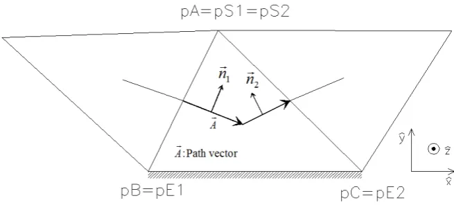
[image:3.595.133.468.397.494.2]

When using the Maxwell stress tensor to calculate the electromagnetic force, the magnetic flux density should be calculated with the normal outward vector. The definition of the normal outward unit vector in the integration path and the components of the vector are shown in Figure 3. In addition, each component unit vector is derived by the operation of the vector A having the arbitrary physical quantity and the normal unit vector.

[image:3.595.131.459.581.729.2]

The arbitrary vector A, the normal vector and the cross product are as follows.

y

n

x

n

n

ˆ

=

_x

ˆ

+

_y

ˆ

(17)

x

A

y

A

y

A

x

A

z

A

z

n

=

ˆ

×

=

ˆ

×

(

x

ˆ

+

y

ˆ

)

=

x

ˆ

+

y

ˆ





(18) 2 2

ˆ

ˆ

ˆ

y x x y

A

A

y

A

x

A

n

+

+

−

=

(19) Here, 2 2 y x y x

A

A

A

n

+

−

=

_, 2 2 y x x y

A

A

A

n

+

=

₍₂₀₎

We will now describe how to apply the virtual displacement method in the finite element method. The virtual displacement method is a method of calculating the electromagnetic force based on energy. When the virtual displacement p is considered, the electromagnetic force F in the p direction can be obtained by calculating the change amount of the total system magnetic field energy. When the magnetic field energy is differentiated in the finite element method, it is necessary to differentiate the system matrix inevitably.

If we express the magnetic force using the virtual displacement method as follows, and the magnetic flux density is represented by the magnetic vector potential A, the following is obtained in the two-dimensional space.

p

W

F

_p

∂

∂

−

=

(21)

[

]

_∑

[

]

∑∫

∫

=

+

=

∆

+

=

∆ 2 2 2 2 2

2

1

1

2

1

2

1

y x e y x

S

dS

B

B

dS

B

B

B

W

µ

µ

µ

(22)

The square of the magnetic flux density and magnetic flux density used in the above energy equation can be expressed in each element as follows.

y

x

A

x

y

A

A

B

z

_ˆ

z

_

_ˆ











∂

∂

−













∂

∂

=

⋅

∇

=





(23)

[

]

{

}









































+

+

+

+

+

+

∆

=

+

3 2 1 2 3 2 3 3 2 3 2 2 2 2 2 3 1 3 1 2 1 2 1 2 1 2 1 3 2 1 2 2 2

.

4

1

A

A

A

d

c

sym

d

d

c

c

d

c

d

d

c

c

d

d

c

c

d

c

A

A

A

B

B

x y (24)

{ }

[ ]{ }

_∑

{ }

[ ]{ }

∑

=

=

A

K

A

A

S

A

W

T e T

8

1

2

1

,

[ ]

S

=

8

µ

e

∆

e

[ ]

K

(25)

When the partial differential form is taken for each component in the virtual displacement method, the components of the magnetic force are as follows.

∑













∆

∂

∂

−

=

e e T x

A

S

A

x

F

{

}

[

]

{

}

8

1

(26)

∑













∆

∂

∂

−

=

e e T y

A

S

A

y

F

{

}

[

]

{

}

8

1

Here, the partial differentiations of the triangular element and the matrix are respectively as follows.

∑

=

∂

∂

∂

∂

=

∂

∂

3

1 i

i

i

x

x

x

V

x

V

∑

=

∂

∂

∂

∂

=

∂

∂

3

1 i

i

i

y

y

y

V

y

V

(28)

∑

=

∂

∂

∂

∂

=

∂

∂

3

1 i

i

i

x

x

x

S

x

S

∑

=

∂

∂

∂

∂

=

∂

∂

3

1 i

i

i

y

y

y

S

y

S

(29)

In this case,

∂

x

i

/

∂

x

is '1' if the i-th node on the element is on the boundary, and '0' otherwise. When using the virtual displacement method to calculate the electromagnetic force, the electromagnetic force of all the elements except the element that touches the boundary of the force body becomes '0'. Therefore, as in the Maxwell stress method, it is possible to obtain the total electromagnetism of the object by integrating the electromagnetic force of the element in contact with the boundary.

3. Numerical Application

[image:5.595.79.293.110.180.2]

The electromagnetic force calculation method using Maxwell stress tensor and the principle of virtual displacement is verified by comparing with the results of axisymmetric three-dimensional analysis in which has analytic solutions.

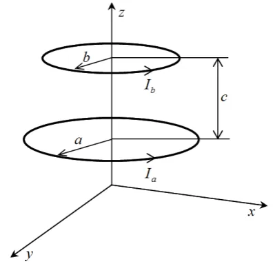
Figure 4. Dipole model with an analytic solution for the verification of the proposed method

Figure 4 shows the proposed method for the coaxial circular loop with two currents. This model has an analytic solution and is also called a dipole model. This model is modeled by three-dimensional axial symmetry and compared with the results of the proposed method. The structural dimensions a, b, and c of the analytical model were 0.1 m, respectively, and the current through the circular loop was 594.5 A.

In order to obtain this model analytically, it is assumed that there is no cross - sectional area of the magnetic dipole. However, in the finite element method, it is impossible to interpret it unless there is an area or a volume in each area. Therefore, it is applied only to the three - dimensional axisymmetric problem which can be modeled as a two - dimensional problem. The electromagnetic force between two magnetic dipoles on the coaxial axis can be analytically determined by the following equation.

   

 

− +

− + + +

+

= ( ) ( )

) ( )

( 2 2 1 1

2 2 2

2

2 _{a b c} E k K k

c b a

c b a

c I I

F a b

z

µ

(28)

where,

∫

−

=

/2

0

2 1

1

)

1

sin

(

k

π

k

φ

d

φ

E

(29)

∫

₋

=

/2

0 2

1 1

sin

1

1

)

(

π

φ

φ

d

k

k

K

₍₃₀₎

2 2 2

1

)

(

4

c

b

a

ab

k

+

+

=

(31)

Here,

E

(

k

1

)

and

K

(

k

1

)

are calculated by Legendre

elliptic integration.

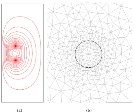
[image:5.595.306.542.290.450.2]

Figure 5 shows the equi-potential line and mesh around the upper cable for numerical analysis of coaxial cable. Table 1 represents the results of force calculation using three kinds of method. Although the numerical analysis results are a little bit large, they agree with the analytical solution. The error of the numerical analysis method is very slight, about 0.19% in both cases.

Table 1. Force comparison of magnetic dipole according to calculation method

Magnetic force

Analytic Solution.

Principle of virtual displacement

Maxwell stress tensor

z

[image:5.595.73.273.424.617.2]

(a) (b)

Figure 5. (a)Equi-potential line and (b)mesh around the upper cable in numerical analysis

4. Conclusions

In this paper, we describe the methodology for analyzing electromagnetic fields and calculating electromagnetic force using finite element method. In general, the algorithm is described from the standpoint of a programmer who codes the Maxwell stress tensor and the principle of virtual work used for electromagnetic force calculation. The Maxwell stress tensor method describes the integral path when calculating the force. Also, when applying the principle of the virtual displacement, we mentioned that the matrix is differentiated. In addition, three dimensional models with analytical solution were selected and compared with the proposed method.

Acknowledgements

This paper was supported by Joongbu University Research & Development Fund, in 2019.

REFERENCES

[1] Salon, SJ. Finite element analysis of electrical machines (Vol. 101). Boston USA: Kluwer academic publishers; 1995.

[2] Jin, Jian-Ming. The finite element method in electromagnetics. John Wiley & Sons, 2015.

[3] Brebbia, Carlos Alberto, and Stephen Walker. Boundary element techniques in engineering. Elsevier, 2016.

[4] Monzon, Lorena MA, John Michael David Coey. Magnetic fields in electrochemistry: The Lorentz force. A mini-review. Electrochemistry Communications. 2014; 42:38-41.

[5] Freschi, Fabio, Maurizio Repetto. Natural choice of integration surface for Maxwell stress tensor computation. IEEE Transactions on Magnetics. 2013; 49(5):1717-1720. [6] Mahmud, M. A. R., Rahman, M. M., & Miah, M. S.

Performance Analysis of Routing Protocols for CBR Traffic in Mobile Ad-Hoc Networks. Journal of Information. 2016; 2(1): 1-9.

[7] Mahmudova, S. (2018). Methods of Organizing the Technological Process of Software Development. Review of Information Engineering and Applications, 5(1), 1-11. [8] Malinga, N. G., Masuku, M. B., & Raufu, M. O.

Comparative analysis of technical efficiencies of smallholder vegetable farmers with and without credit access in swazil and the case of the Hhohho region. International Journal of Sustainable Agricultural Research. 2015; 2(4): 133-145.

[9] Messaoudene, I., Belhocine, M. A., Aidel, S., & Djeffal, N. Enhanced Isolation Mimo Antenna with DGS Structures for Long Term Evolution Systems. Review of Computer Engineering Research. 2015; 2(4):71-76.

[10]Fonteyn KA, Belahcen A, Rasilo P, Kouhia R, Arkkio A. Contribution of maxwell stress in air on the deformations of induction machines. 2010 International Conference on Electrical Machines and Systems. IEEE. 2010.

[11]Bermúdez A, Rodríguez AL, Villar I. Extended formulas to compute resultant and contact electromagnetic force and torque from Maxwell stress tensors. IEEE Transactions on Magnetics. 2017; 53(4):1-9.

[12]Coulomb J, Meunier G. Finite element implementation of virtual work principle for magnetic or electric force and torque computation. IEEE Transactions on magnetics. 1984; 20(5):1894-1896.

[13]Coulomb J. A methodology for the determination of global electromechanical quantities from a finite element analysis and its application to the evaluation of magnetic forces, torques and stiffness. IEEE Transactions on Magnetics. 1983;19(6): 2514-2519.

[image:6.595.59.293.75.271.2]