An Overview of Inductive Learning Algorithms

An

Overview of

Inductive

Learning Algorithms

Amal M. AlMana

College of Computer and Information Sciences Information Systems Department

King Saud University Riyadh, Saudi Arabia

Mehmet Sabih Aksoy,

College of Computer and Information Sciences Information Systems Department

King Saud University Riyadh, Saudi Arabia

ABSTRACT

Inductive learning enables the system to recognize patterns and regularities in previous knowledge or training data and extract the general rules from them. In literature there are proposed two main categories of inductive learning methods and techniques. Divide-and-Conquer algorithms also called decision Tree algorithms and Separate-and-Conquer algorithms known as covering algorithms. This paper first briefly describe the concept of decision trees followed by a review of the well known existing decision tree algorithms including description of ID3, C4.5 and CART algorithms. A well known example of covering algorithms is RULe Extraction System (RULES) family. An up to date overview of RULES algorithms, and Rule Extractor-1 algorithm, their solidity as well as shortage are explained and discussed. Finally few application domains of inductive learning are presented.

Keywords

Data Mining, Rules Induction, RULES Family, REX-1, Covering Algorithms, Inductive Learning, ID3, C4.5, CART, and Decision Tree algorithms

1.

INTRODUCTION

A new field of machine learning known as inductive learning has been introduced to help in inducing general rules and predicting future activities [1]. Inductive learning is learning from observation and earlier knowledge by generalization of rules and conclusions. Inductive learning allows for the identification of training data or earlier knowledge patterns and similarities which are then extracted as generalized rules. The identified and extracted generalized rules come to use in reasoning and problem solving[2]. Data mining is one step in the process of knowledge discovery in databases (KDD). It is possible to design automated tools for learning rules from databases by using data mining or other knowledge discovery techniques[3][4]. There is an intersection point between the field of data mining and machine learning as they both extract interesting patterns and knowledge from databases[5]. According to Holsheimer et al. [6], data mining refers to the use of the database as a training set in the learning process.

In inductive learning different methods have been proposed to infer classification rules. These methods and techniques were divided into two main categories: Divide-and-Conquer (Decision Tree) and Separate-and-Conquer (Covering). Divide-and-conquer algorithms, such as ID3, C4.5 and CART are classification techniques that derive the general conclusions using decision tree. Separate-and-Conquer algorithms such as AQ family, CN2 (Clark and Niblett), and RULES (RULe Extraction System) family where rules are directly induced from a give set of training examples[1][7]. A decision tree represents one of the mostly used approaches in inductive machine learning. A set of training examples usually used to form a decision tree [4]. The preference of

decision trees for inductive learning is due to their ease in implementation and comprehension, and the lack of methods for preparation like normalization. Decision tree performance is good and it can function well with large databases. For this reason and due to its efficiency decision tree can handle a huge amount of training examples. Both numerical and categorical data are possible in the decision tree structure. Decision trees generalize in a better way for data instances not yet observed, once examined the attribute value pair in the training data. The better understanding of classification based on the attributes provided. The attribute arrangement on the decision tree is from the information available hence the classification is well laid out. The negative aspect of the decision trees is that the generalized rules given are not always the most generalized. For this reason, some algorithms like AQ family algorithms do not use decision trees. The AQ algorithm family makes use of the disjunction of positive examples feature values [8].

In the arena of divide-and-conquer algorithms, a major issue that arises is the complications with trying to show certain rules in the tree. Specifically, it‟s challenging to induce rules that do not have anything in common with tree attributes, and a further complication is the fact that some attributes that show up are either repetitive or unnecessary[9]. Also, these algorithms caused the replication problem, wherein sub-trees can be repeated on different branches. It is difficult to handle a tree when it gets too big. Using divide-and-conquer methods on a large tree might lead to unnecessary confusion[7].

As a consequence, researchers have lately tried improving covering algorithms to compare or exceed the results of divide-and-conquer attempts. It is better to induce the rules directly from the dataset itself instead of inducing them from a decision tree structure which is summarized into four main properties according to Kurgan et al. [10] . Firstly, using representation such as “IF…THEN” makes the rules more easily understood by people. It is also a proven fact that rule learning is a more effective method than using decision trees. Moreover, the derived rules can be used and stored easily in any expert system or any knowledge-based system. Lastly, it is also easier to study and make changes to rules that have been induced without affecting other rules because they are independent of each other[10].

2.

DIVIDE AND

CONQURE

ALGORITHMS

A brief explanation of the concept of decision tree and the well known divide and conqure algorithms such as ID3, C4.5 and CART are presented below.

2.1. Decision Tree

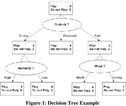
Decision trees, according to Mitchell[11], categorize instances by arranging them form the root to a particular leaf node down the tree. This acts as the categorization of instances. Any node in the tree represents a test of some attribute of the instance while each descending branch from the node, will represent a possible attribute value. The figure below is an example of a decision tree constructed based on the attribute named outlook. The outlook attribute has three values overcast, sunny, and rain. Some values have sub trees like rain and sunny values in figure 1. Classification of examples into distinct set of probable groupings, are often termed as classification problems [8][11].

Figure 1: Decision Tree Example

The first step achieved by the tree models is the categorization into groups of the observations. The process that follows after achieving the groups form the categorization process is the scoring of these particular groups. Classification trees and regression trees are the two categories of tree models. A regression tress has a continuous response variable but the classification trees, have a quantitative or qualitative categorical response variable. It is possible to give the definition of tree models as a recursive procedural process where n statistical units, in a set, put into groups. The process of putting the units into groups is by division dependent on a given division rule, and it is progressive. The aim of the division rule is homogeneity maximization or the response variable purity measure in its group as obtained. The division rule institutes a way of partitioning the observations. Each division procedure in the process is dependent on the explanatory variable to split and the splitting rule required, knowing the division rule applicable. A final partition of the observations is the main result of any decision tree [3].

2.2 Decision Tree Learning Algorithms

Among the many algorithms for decision trees creation, ID3 and C4.5 by J. R. Quinlan, are the two mostly used. Another famous algorithm is CART by Breiman. A brief explanation of each one of them is presented below.

2.2.1 ID3 Algorithm

Ross Quinlan created Iterative Dichotomiser 3 algorithm in 1986. It is also known as ID3 algorithm. It is among the algorithms earlier stated. ID3 is based on Hunt‟s algorithm. It is a simple decision tree learning algorithm. In the iterative inductive approach ID3 is used to classify objects[8]. The whole idea in the buildup of the ID3 algorithm is accomplished through the top down search of particular sets to examine every attribute at each node in the tree [12][13]. Here, a metric, Information gain, comes into play for the purpose of attribute selection. Attribute selection is the main part of classification of given sets. Information gain enables for the measure of the relevance of the questions asked. This allows for the minimization of the questions needed for the classification of a learning set. The choice that ID3 makes on the splitting attribute depends on the information gain measure. Claude Shannon came up with the idea of measuring information gain by entropy in 1948[8][13].

ID3 has a preference for the trees generated. Once generated, the tree should be shorter and near the top of the tree is where attributes with lower entropies should be [2]. In building the tree models, ID3 accepts categorical attribute. This is the only process where ID3 accepts them. ID3 algorithm implement decision tree serially. However in the existence of noise ID3 does not give accurate results. For this reason, ID3 has to perform a thorough processing of data before its use in tree model building. These decision trees are mostly used for the decision making purpose [8][14].The figure below shows the basic implementation technique of ID3 algorithm as presented in [2].

Figure2: ID3 algorithm

There are problems with ID3 algorithm. The resultant decision tree over fitting the training example is one problem. This is as a result of the procedural splitting in the attempt of individual split optimization instead of the whole tree optimization [4]. The outcome of this process is decision trees that are too precise from the use of conditions that are pointless or irrelevant. There is a repercussion to this outcome. This is the interference of the categorization of unknown examples or those examples with incomplete attributes values. Usually, pruning is used to reduce over fit in decision trees. However, this procedure may not work efficiently for an inadequate data set that demands probabilistic as opposed to categorical classification [15].

1 .For each uncategorized attribute, its entropy would be calculated with respect to the categorized attribute, or conclusion.

2. The attribute with lowest entropy would be selected. 3. The data would be divided into sets according to the attribute‟s value. For example, if the attribute „Size‟ was chosen, and the values for „Size‟ were „big‟, „medium‟ and „small, therefore three sets would be created, divided by these values.

4. A tree with branches that represent the sets would be constructed. For the above example, three branches would be created where first branch would be „big‟, second branch would be „medium‟ and third branch would be „small‟.

5. Step 1 would be repeated for each branch, but the already selected attribute would be removed and the data used was only the data that exists in the sets.

2.2.2 C4.5 Algorithm

Ross Quinlan, 1993, developed an upgraded algorithm of ID3. C4.5 is the ID3 upgrade. C4.5 is similar to its predecessor in that is based on Hunt‟s algorithm and it has a serial implementation. Tree pruning in C4.5 is after its creation. Once created, it returns through the tree created and tries to eliminate irrelevant branches by substituting them with leaf nodes hence the error rate decreases [16].

Both continuous and categorical attributes are acceptable in tree model building in C4.5, unlike in ID3. It uses categorization to tackle continuous attributes. This categorization is done by creating a threshold and separating the attributes based on their position in reference to this threshold [17][18]. Determination of the best splitting attribute, like in ID3, is at each tree node through the sorting of data. In C4.5, splitting attribute evaluation is by the gain ratio impurity method [13]. C4.5 can work with training data with attributes missing values. It allows for the missing values representation as “?”. It also works with attributes with different costs. In gain ratio and entropy calculations, C4.5 ignores the missing value attributes [16].

2.2.3 CART Algorithm

Classification and regression tree algorithm also known as CART is a development by Breiman in 1984. From its name, it is able to generate classification and regression model trees. CART binary splits attributes in the building of the classification trees. Like ID3 and C4.5, it is based on Hunt‟s algorithm and can apply serial implementation [18].

In CART decision tree building, categorical and continuous attributes are both acceptable. It is similar to C4.5 in that it can work with missing attributes in data. CART applies the Gini index splitting measure to determine the splitting attribute for the decision tree construction[13]. From its use of the binary splitting of attributes, it gives binary splits hence binary decision trees. This is different from ID3 and C4.5 split production. Unlike ID3 and C4.5 algorithms, Gini Index measure does not use probabilistic assumptions. Therefore, the unreliable branches are pruned following the cost complexity. This improves the tree‟s accuracy [17][18].

3. SEPARATE AND CONQUER

ALGORITHMS

Separate-and-Conquer algorithms such as AQ family, CN2, Rule Extractor-1 and RULES family of algorithms where rules are directly induced from a give set of training examples.

3.1. RULES Family of Algorithms

Below is a brief description of all versions of Rules Family of Algorithms.

3.1.1. RULES-1

RULES-1 (RULe Extraction System-1) also known as RULES algorithm was developed by Pham and Aksoy[19][20]. An implementation of RULES-1 extracts rules for objects in similar sets of classes. Each object has its own attributes and values, which makes them individual. Each condition consists of an attribute and value pair, so for example, if an object has Na as the number of attributes, the rule may fall between one and Na conditions. In a collection of objects all of their values and attributes construct an array. The size of the array is equal to the total number of all values. At most, there can be Na iterations in the rule-forming procedure[19][20].

In the initial loop, the system examines every element to see if it is able to be part of a rule with that element as the condition. It can help form a rule if any given element in that loop applies to a single class. If, however, it applies to more than one class, it is overlooked in favor of the next potential element. Once RULES-1 has checked all elements, it rechecks all examples against the candidate rule to ensure everything is in place. If any examples remain that is unclassified, a new array is constructed containing all unclassified examples and the next iteration of the procedure is initiated. If no more unclassified examples, the procedure is finished. This continues until everything is classified properly or all iterations equal Na[19][20]. This process can be seen in the flowchart below in figure 3[19].

Figure3: Flow chart of RULES

3.1.2. RULES-2

After creating 1, Pham and Aksoy invented RULES-2 in 1995. RULES-RULES-2 is essentially similar to RULES-1 in terms of how it derives rules; however the only difference is that RULES-2 considers the value of one unclassified example to produce a rule for classifying that example instead of considering the values of all unclassified examples in each loop. As a result RULES-2 is able to operate faster. It also gives the user some control over how many rules need to be extracted. Another advantage is RULES-2‟s ability to compute with examples that aren‟t complete, and to handle numeric and nominal values while filtering out examples that aren‟t relevant and automatically avoids irrelevant conditions[20].

3.1.3. RULES-3

RULES-3 was the succeeding version, which built on the advantages of the systems that came before and also introduced new features, such as more compact rule sets and ways to adjust how precise the rules extracted need to be. Users of RULES-3 can define the minimum number of conditions need to exist to create a rule. There are advantages to this – the rules will be more exact, and not as many search operations will be needed to find the correct rule set[20]. This process can be summarized as below in figure 4[21].

Figure4: RULES-3 algorithm

3.1.4. RULES3-Plus

In 1997 Pham and Dimov built upon RULES-3‟s ability to form rules in their creation of RULES-3 PLUS algorithm [22]. RULES-3 Plus is more efficient than RULES-3 in searching out rules, it applies the beam search strategy instead of greedy search and it makes use of the so-called H measure to help with selecting rules according to how correct and general they are.

However, RULES-3 Plus does have its drawbacks – its efficiency is not a foregone conclusion, as it tends to overly-train itself to cover all data. The H measure, as well, is a very complex calculation and it doesn‟t always bring in the most accurate and general results. Although RULES-3 Plus discretised its continuous valued attributes, its discretisation method does not follow any set rules; it is arbitrary and doesn‟t try to find any information in the data, which inhibits RULES-3 Plus‟ ability to learn new rules. A summary of the

rule forming procedure of RULES-3 Plus is presented below in figure 5 [22].

Figure5: Rule forming procedure of RULE-3 Plus

3.1.5. RULES-4

RULES-4 [23] was created to address the ability to extract rules incrementally in the RULES family byprocessing one example at a time. Pham and Dimov developed RULES-4 in 1997 as the first incremental learning algorithm under the RULES family. They invented it to be a variation on RULES-3 Plus, and it has some additional advantages – namely the ability to store training examples in the Short Term Memory (STM) when they become available and ready. Another advantage of RULES-4 is the ability to let the user specify the size of the STM storage used in the creation of the rules. When that memory is full, RULES-4 has the ability to draw

Step 1 Quantize attributes that have numerical values.

Step 2 Select an unclassified example and form array SETAV.

Step 3 Initialize arrays PRSET and T_PRSET (PRSET and T_PRSET will consist of mPREST expressions with null

conditions and zero H measures) and set nco=0. Step 4 IF nco < na

THEN nco = nco + 1 and set m = 0;

ELSE the example itself is taken as a rule and go to Step 7.

Step 5 DO

m=m+ 1;

Form an array of expressions (T_EXP). The elements of this array are combinations of expression m in PRSET with conditions from SETAV that differ from the conditions already included in the expression m (the number of elements in T_EXP is: na - nco. Set

k = 1; DO

k=k+ I;

Compute the H measure of expression k in T_EXP;

IF its H measure is higher than the H measure of any expression in T_PRSET THEN replace the expression having the lowest H measure with expression k;

WHILE k < na - nco ;

Discard the array T_EXP; WHILE m < mPREST

Step 6 IF there are consistent expressions in T_PRSET THEN choose as a rule the expression that has the highest H measure and discard the others;

Mark the examples covered by this rule as classified;

Go to Step 7;

ELSE copy T_PRSET into PRSET; Initialize T_PRSET and go to Step 4.

Step 7 IF there are no more unclassified examples THEN STOP;

ELSE go to Step 2.

(Note: nco = number of conditions, na = number of Attributes,

T_EXP= a temporary array of expressions, mPRSET= number

of expressions stored in PRSET and its given by the user, T_PRSET= a temporary array of partial rules of the same dimension as PRSET).

Step 1 Define ranges for the attributes, which have numerical values and assign labels to those ranges

Step 2 Set the minimum number of conditions (Ncmin) for each rule

Step 3 Take an unclassified example

Step 4 Nc=Ncmin–1

Step 5 If Nc<Na then Nc=Nc+1

Step 6 Take all values or labels contained in the example

Step 7 Form objects, which are combinations of Nc values or labels taken from the values or labels obtained in Step 6

Step 8 If at least one of the objects belongs to a unique class then form rules with those objects; ELSE go to Step 5

Step 9 Select the rule, which classifies the highest number of examples

Step 10 Remove examples classified by the selected rule

Step 11 If there are no more unclassified examples then STOP; ELSE go to Step 3.

on RULES-3 Plus‟ knowledge to create new rules. Pham and Dimov explain the incremental algorithm in figure 6.

Figure6: The incremental induction procedure of RULES-4

STM always empty and it‟s initialized with a set of examined examples. LTM contained the previously extracted rules or some initial rules defined by the user[23].

3.1.6. RULES-5

Pham et al. [24] invented RULES-5 in 2003 which built on the advantages of RULES-3 Plus . They tried to overcome some insufficiencies of RULES-3 Plus algorithm in their newly developed algorithm called RULES-5. It implements a method to manage continuous attributes so there is no need for quantization[24]. Choosing the condition and the procedure of handling continues attributes are the main process in RULES-5 algorithm. The authors explain this core process as follows: The process of rule extraction in RuleS-5 consider only the conditions except the closest example (CE) that is covered by the extracted rule and does not belong to the target class. Any data set may include both continues and discrete attributes. In order to calculate CE, a measure is used to compute the distance between any two examples in the data set whether it includes discrete attributes or continues ones. The main advantage that distinguishes RULES-5 from previous RULES algorithms is its ability to generate fewer rules in a very accurate manner. As a result it takes shorter training time and searching time[20].

3.1.7. RULES-6

RULES-6 was developed by Pham and Afify [25] in 2005 using RULES-3 Plus as a basis. RULES-6 is a quick way of finding IF-THEN rules from given examples; it is also simpler in its evaluations of rules and how it handles continuous attributes. Because Pham and Afify developed RULES-6 to build on and improve RULES-3 Plus by adding the ability to

handle noise in dataset, RULES-6 is both more accurate and easier to use, and it doesn‟t suffer the same slowdowns in the learning process because it doesn‟t get bogged down in useless details. Making it even more effective, RULES-6 uses simpler criteria for qualifying rules and checking continuous values in the algorithms which led to a further improvement in the performance of the algorithm. Figure 7 describes the pseudo code of RULES-6. A pruned general to specific search is carried out by Induce_One_Rule procedure to search for rules [25].

Figure7: Pseudo code description of RULES-6

3.1.8. RULES3- EXT:

In 2010 Mathkour [26] developed a new inductive learning algorithm called RULES3-EXT. many disadvantages exist in RULES-3, RULES3-EXT was created to address them efficiently. The main advantages of RULES3-EXT are as follows: It is capable of eliminating repetitive examples, allowing users to make changes where needed in attribute order, if any of the extracted rules cannot fully be satisfied by an unseen example the system can partially fire rules, and it can work on a smaller number of required files to extract a knowledge base two files instead of three. The main steps which describe the induction process of RULES3-EXT algorithm are given below in figure 8 [26].

Figure8: RULES3- EXT algorithm

3.1.9. RULES-7

RULES family has extended to Rules-7 [27], also known as RULe Extraction System Version 7 which improves upon its predecessor RULES-6 by fixing some of its drawbacks. RULES7 employs a general to specific beam search on the data set to derive the best rule. It selects sequentially a seed example that is passed by Induce_Rules procedure to the Induce_One_Rule procedure after calculating MS which is the

Step 1 Define ranges for the attributes, which have numerical values and assign labels to those ranges.

Step 2 Set the minimum number of conditions (Ncmin) for each rule.

Step 3 Take an unclassified example.

Step 4 Nc=Ncmin-1

Step 5 If Nc<Na then Nc=Nc+1

Step 6 Take all values or labels contained in the example.

Step 7 Form objects, which are combinations of Nc values or labels taken from the values or labels obtained in Step 6.

Step 8 If at least one of the objects belongs to a unique class then form rules with those objects; ELSE go to Step 5.

Step 9 Select the rule, which classifies the highest number of examples.

Step 10 Remove examples classified by the selected rule.

Step 11 If there are no more unclassified examples then STOP; ELSE go to Step 3.

(Note: Nc: number of conditions, Na: number of attributes).

Procedure Induce_Rules (TrainingSet, BeamWidth) RuleSet = ∅

While all the examples in the TrainingSet are not covered

Do

Take a seed example s that has not yet been covered Rule = Induce_One_Rule (s, TrainingSet, BeamWidth) Mark the examples covered by Rule as covered RuleSet = RuleSet ∪ {Rule}

End While Return RuleSet

End Input: Short-Term Memory (STM), Long-Term Memory,

ranges of values for numerical attributes, frequency distribution of examples among classes, one new example.

Output: STM, LTM, updated ranges of values for numerical attributes, updated frequency distribution of examples among classes.

Step 1 Update the frequency distribution of examples among classes.

Step 2 Test, whether the numerical attributes are within their existing ranges and if not update the ranges.

Step 3.Test whether there are rules in the LTM that classify or misclassify the new example and simultaneously update their accuracy measures (A measures) and H measures.

Step 4 Prune the LTM by removing the rules for which the A measure is lower than a given prespecified level (threshold).

Step 5 IF the number of examples in the STM is less than a prespecified limit THEN add the example to the STM ELSE IF there are no rules in the LTM that classify the new example THEN replace an example from the STM that belongs to the class with the largest number of presentatives in the STM by the new example.

minimum number of instances to be covered by the ParentRule. The ParentRuleSet and ChildRuleSet both are initialized to Null.

A rule with antecedent is created by the procedure called SETAV marking all conditions in the rule antecedent as not existing. BestRule (BR) is the most general rule developed by SETAV procedure and it is included in to the ParentRuleSet for specialization. Now the loop keeps iterating until the ChildRuleSet is empty and there are no more rules left in it to be copied into ParentRuleSet. The RULES-7 algorithm only considers those rules in the ParentRuleSet which have coverage more than MS. Once the criterion has been fulfilled, the rule adds new “Valid” condition to it by simply change the “exist” flag of the condition from its default value “no” to “yes.” [27]. This rule called ChilRule (CR) and it will pass through a check for rule duplication to make sure that ChildRuleSet is free from any kind of duplication. Different control structure has been used in RULES-7 to fix some flaws in RULES-6. Since duplicate rule check has already been carried out, algorithm does not require another step at the end to remove duplicate rules from ChildRuleSet which helps save significant time as compared to RULES-6[27]. A flowchart of RULES-7 is given in figure 9.

Figure 9: A simplified description of RULES-7

3.1.10. RULES-8

In 2012 Pham [28] developed a new rule induction algorithm called RULES-8 for handling discrete and continuous variables without the need for any data pre-processing. It also has the ability to deal with noisy data in the data set. RULES-8 has been proposed to address the deficiencies of its predecessors by selecting a candidate attribute-value instead of a seed example to form a new rule. It chooses the candidate attribute-value to make sure the generated rule is the best rule. The conditions selection is based on applying specific heuristic H measure. The conjunction of conditions is created by incrementally appending conditions based on H measure.

This measure helps assess the information content of each newly formed rule. There is also an improved simplification technique applied on rules to produce more compact rule sets and reduce the overlapping between rules.

Seed attribute-value is considered as a candidate condition which when applied to a rule is capable of covering most examples. Different from its predecessors in the RULES family, RULES-8 algorithm first selects a seed attribute-value and then employs a specialisation process to find a general rule by incrementally adding new conditions to them. Figure 10 describes the rule forming procedure of RuLES-8 algorithm[28].

Step 1: Select randomly one uncovered attribute-value from each attribute to form an array SETAV = [A.1 A.2 .. A.j ] , then

mark them in the training set T.

Step 2: Form array expression T_EXP from SETAV

Step 3: Compute H measure for each expression in T_EXP and sort them out according to the accuracy of expressions and then add them to the PRSET (highest H measure). If the H measure of the newly formed rule is higher than the H measure on any rules in the PRSET, the new rule replaces the rule having the lowest H measure.

Step 4: Select an expression with a potential condition (Aij)

having the highest H measure to find the seed attribute-value (Ais)

IF the expression having the highest H measure covers correctly all covering example

THEN the potential condition (Aij) is selected as a

seed attribute-value (Ais).

Assume that it covers n examples.

- Removes this expression from the PRSET - Go to step 7

ELSE go to step 5

Step 5: Check uncovered attribute-values

IF there are not uncovered attribute-values THEN Stop

ELSE check uncovered attribute-values.

IF there are uncovered attribute-values that have not been marked

THEN go to step 1. ELSE go to step 6.

Step 6: Form a new array SETAV by combining the potential attribute-value with other attribute value in the same example SETAV = [Aij + Ai1 ; Aij + Ai2 ;.. Aij + Aik ].

Go to step 2.

Step 7: Form a set of conjunctions of condition SETCC by combining is Ais with other attribute-values, SETCC = [Ais +

Ai1 ; Ais + Ai2 ;.. Ais + Aik ].

Step 8: Form array rule Temporary Rule Set (T_RSET) from SETCC.

Step 9: Compute H measure for each expression of T_RSET and sort them out according to the consistency of expressions and then add them to the NRSET (highest H measure). If the H measure of the newly formed rule is higher than the H measure on any rules in the NRSET, the new rule replaces the rule having the lowest H measure.

Step 10: Select an expression with the conjunction of conditions (A isc ) having the highest H measure to test the consistency. Assume that it covers m examples

IF m> n THEN A isc is considered as a new seed attribute-value

Go to step 6

Figure 10: A pseudo-code description of RULES-8 rule forming procedure

3.2. RULE EXTRACTOR-1

REX-1 (Rule Extractor-1) was created to acquire IF-THEN from given examples. It is an algorithm inventive for Inductive Learning and to dismiss the pitfalls encountered in the RULES family algorithms. The entropy value is used to give more value to more important attributes. The process of rules induction in REX-1 is as follows: REX-1 calculates basic entropy values and recalculated entropy values, then sets the attributes in ascending order to process the lowest entropy values first. The REX-1 algorithm is described below in figure 11 [29].

Figure11: REX-1 algorithm

4. INDUCTIVE LEARNING

APPLICATIONS

Inductive learning algorithms are domain independent and can be used in any task involving classification or pattern recognition. Some of them are summarized below[30].

4.1. Education

Research in data mining for its use in education is on the rise. This new emerging field, called Educational Data Mining (EDM). Developing methods that discover and extract knowledge from data generating from educational environments is the main concern of EDM[31]. Decision Trees, Neural Networks, Naïve Bayes, K- Nearest neighbor, and many other techniques can be used in EDM. By the application of this technique, there is the discovery of different knowledge kind such as classifications, association rules, and clustering. The extracted knowledge can be used to make a number of predictions. For instance it can be used to predict student enrolment in a certain course, discovery of

abnormal values in the student result slips, and selection of the most suitable course for the students based on their past strengths and skills. Moreover, they can help advice the students on additional courses they should take to boost their performance [12][32].

There exist several decision trees construction algorithms and they are widely used of all machine learning aspects especially in EDM. Examples of the mostly used algorithms in EDM are ID3, C4.5, CART, CHAID, QUEST, GUIDE, CRUISE, CTREE and ASSISTANT. J. Ross Quinlan's ID3 and its successor, C4.5, are among the most widely used decision tree algorithms in the machine learning community [33]. C4.5 and ID3 are similar in how they act but C4.5 has improved behaviors in comparison to ID3.ID3 algorithm bases it selection of the best attribute information gain and on entropy concept. C4.5 handles uncertain data. This comes at the cost of a high rate of classification error. CART is another well known algorithm which divides its data in to two subsets recursively. This makes the data in one subset more homogeneous than the data in the other subset. CART will repeat the process of splitting till a stopping condition is achieved or until the homogeneity norm is reached [3].

4.2. Making Credit Decisions

Loan companies often use questionnaires to collect information about credit applicants in order to determine their credit eligibility. This process used to be manual but has been automated to some extent. For example, American Express UK used a statistical decision procedure based on discriminate analysis to reject applicants below a specific threshold while accepting those exceeding another one. The remaining fell into a "borderline" region and was switched to loan officers for further review. However, loan officers were accurate in predicting potential default by borderline applicants no more than 50% of the time.

These findings inspired American Express UK to try methods such as machine learning to improve decision-making processes. Michie and his colleagues used an induction method to produce a decision tree that made accurate predictions about 70% of the borderline applicants. It does not only improve the accuracy but it helps the company to provide explanations to the applicants [34].

5. CONCLUSION AND FUTURE WORK

Inductive learning enables the system to recognize regularities and patterns in previous knowledge or training data and extract the general rules from them. This paper presented an overview of main inductive learning concepts as well as brief descriptions of existing algorithms. Many classification algorithms have been discussed in the literature but decision tree is the most commonly used tool due to ease of implementation as well as being easier to understand than other classification algorithms. The ID3, C4.5 and CART decision tree algorithms has been explained one by one. To exceed the results of divide-and-conquer attempts researchers have tried to improve covering algorithms. It is preferable to infer rules directly from the dataset itself instead of inferring them from a decision tree. The algorithm of RULES family is used to induce a set of classification rules from a collection of training examples for objects belonging to one known class. A brief description of RULES family is presented including: RULES1, RULES2, RULES3, RULES3-Plus, RULES4, RULES5, RULES6, RULES3-EXT, RULES7 and RULES8. Each version has certain new features to overcome the shortcomings of the previous versions.

Step 1 In a given example set, the entropy is computed for each value and each attribute.

Step 2 Reformulated entropy values are computed. (The entropy value of each attribute is multiplied with the number of the values of the attribute).

Step 3 The reformulated entropy values are stored in ascending manner and the example set is reformed based on the sorting.

Step 4 Odd number (n=1) combinations of the values in each example are selected. Any value of which entropy equals zero for n=1 may be selected as a rule. These values are converted into rules. The classified examples are marked.

Step 5 Go to step 8.

Step 6 Beginning from the first unclassified example, combinations with n values are formed by taking only one attribute from the values of attributes.

Step 7 Each combination is applied to all of the examples in the set of examples. From the values composed of n combinations, those matching with only one class are converted into a rule. The classified examples are marked.

Step 8 IF all of the examples are classified THEN go to step 11.

Step 9 Perform n=n+1 expression.

Step 10 IF n<N THEN go to step 6.

Step 11 IF there are more than one rule representing the same example, the most general one is selected.

Step 12 END.

The objectives behind the research included surveying current inductive learning methods and extending RULES family of algorithms by developing a new simple rule induction algorithm that overcomes certain shortcomings of its predecessors. While I have achieved the first objective behind the research, my future work will be primarily focused on achieving the second goal. It is very important to invent new algorithms or improve current ones to achieve more reliable results. Therefore, my Initial specifications of the newly developed rule induction algorithm but not limited to the following: Generate a compact rule sets for discrete outputs, Handling of discrete and continuous inputs, the ability to deal with noisy examples without increasing the number of rules, the ability to deal with incomplete examples, and improve rule forming processes where possible.

6. REFERENCES

[1] H. A. ELGIBREEN and M. S. AKSOY, “RULES – TL : A SIMPLE AND IMPROVED RULES,” J. Theor. Appl. Inf. Technol., vol. 47, no. 1, 2013.

[2] A. H. Mohamed and M. H. S. Bin Jahabar, “Implementation and Comparison of Inductive Learning Algorithms on Timetabling,” Int. J. Inf. Technol., vol. 12, no. 7, pp. 97–113, 2006.

[3] A. Trnka, “Classification and Regression Trees as a Part of Data Mining in Six Sigma Methodology,” Proc. World Congr. Eng. Comput. Sci., vol. I, 2010.

[4] M. R. ; Tolun and S. M. Abu-Soud, “An Inductive Learning Algorithm for Production Rule Discovery,” Department of Computer Engineering Middle East Technical University. Ankara, Turkey, pp. 1–19, 2007. [5] J. S. Deogun, V. V Raghavan, A. Sarkar, and H. Sever,

“Data Mining : Research Trends , Challenges , and Applications,” in in in Roughs Sets and Data Mining: Analysis of Imprecise Data, Kluwer Academic Publishers, 1997, pp. 9–45.

[6] M. ; S. A. Holsheimer, “Data Mining - The Search for Knowledge in Databases,” Amsterdam, The Netherlands, 1991.

[7] lan H. Witten and E. Frank, Data Mining: Practical Machine Learning Tools and Techniques, 2nd editio. Morgan Kaufmann, 2005.

[8] A. Bahety, “Extension and Evaluation of ID3 – Decision Tree Algorithm.” University of Maryland, College Park, pp. 1–8.

[9] F. Stahl, M. Bramer, and M. Adda, “PMCRI : A Parallel Modular Classification Rule Induction Framework,” in in Machine Learning and Data Mining in Pattern Recognition, Springer Berlin Heidelberg, 2009, pp. 148– 162.

[10] L. A. Kurgan, K. J. Cios, and S. Dick, “Highly scalable and robust rule learner: performance evaluation and comparison.,” IEEE Trans. Syst. Man. Cybern. B. Cybern., vol. 36, no. 1, pp. 32–53, Feb. 2006.

[11] T. M. Mitchell, “Decision Tree Learning,” in in Machine Learning, Singapore: McGraw- Hill, 1997, pp. 52–80. [12] B. K. Baradwaj and P. Saurabh, “Mining Educational

Data to Analyze Students‟ Performance,” Int. J. Adv. Comput. Sci. Appl., vol. 2, no. 6, pp. 63–69, 2011.

[13] A. Rathee and R. prakash Mathur, “Survey on Decision Tree Classification algorithms for the Evaluation of Student Performance,” Int. J. Comput. Technol., vol. 4, no. 2, pp. 244–247, 2013.

[14] R. Bhardwaj and S. Vatta, “Implementation of ID3 Algorithm,” Int. J. Adv. Res. Comput. Sci. Softw. Eng., vol. 3, no. 6, pp. 845–851, 2013.

[15] L. Breiman, J. H. Friedman, R. A. Olshen, and C. J. Stone, “Classification and regression trees,” vol. 57, no. 1. Monterey, Calif.:Wadsworth and Brooks, Feb-1984.

[16] T. Verma, S. Raj, M. A. Khan, and P. Modi, “Literacy Rate Analysis,” Int. J. Sci. Eng. Res., vol. 3, no. 7, pp. 1– 4, 2012.

[17] S. K. Yadav and S. Pal, “Data Mining : A Prediction for Performance Improvement of Engineering Students using Classification,” World Comput. Sci. Inf. Technol. J., vol. 2, no. 2, pp. 51–56, 2012.

[18] X. Wu, V. Kumar, J. R. Quinlan, J. Ghosh, Q. Yang, H. Motoda, G. J. McLachlan, A. Ng, B. Liu, P. S. Yu, Z.-H. Zhou, M. Steinbach, D. J. Hand, and D. Steinberg, “Top 10 algorithms in data mining,” Knowl. Inf. Syst. , Spriger, vol. 14, no. 1, pp. 1–37, Dec. 2007.

[19] D. T. Pham and M. S. Aksoy, “RULES: A simple rule extraction system,” Expert Syst. Appl., vol. 8, no. 1, pp. 59–65, Jan. 1995.

[20] M. S. Aksoy, “A Review of RULES Family of Algorithms,” Math. Comput. Appl., vol. 13, no. 1, pp. 51–60, 2008.

[21] M. S. Aksoy, H. Mathkour, and B. A. Alasoos, “Performance evaluation of rules-3 induction system on data mining,” Int. J. Innov. Comput. Inf. Control, vol. 6, no. 8, pp. 1–8, 2010.

[22] D. T. Pham and S. S. Dimov, “AN EFFICIENT ALGORITHM FOR AUTOMATIC KNOWLEDGE ACQUISITION,” Pattern Recognit., vol. 30, no. 7, pp. 1137–1143, 1997.

[23] D. T. Pham and S. S. Dimov, “An algorithm for incremental inductive learning,” Proc. Inst. Mech. Eng. Part B J. Eng. Manuf., vol. 211, no. 3, pp. 239–249, Jan. 1997.

[24] D. T. Pham, S. Bigot, and S. S. Dimov, “RULES-5: a rule induction algorithm for classification problems involving continuous attributes,” Proc. Inst. Mech. Eng. Part C J. Mech. Eng. Sci., vol. 217, no. 12, pp. 1273– 1286, Jan. 2003.

[25] D. T. Pham and a. a. Afify, “RULES-6: a simple rule induction algorithm for supporting decision making,” 31st Annu. Conf. IEEE Ind. Electron. Soc. 2005. IECON 2005., p. 6 pp., 2005.

[26] H. I. Mathkour, “RULES3-EXT IMPROVEMENTS ON RULES-3 INDUCTION ALGORITHM,” Math. Comput. Appl., vol. 15, no. 3, pp. 318–324, 2010.

[28] D. T. Pham, “A Novel Rule Induction Algorithm with Improved Handling of Continuous Valued Attributes,” Cardiff University, 2012.

[29] Ö. Akgöbek, Y. S. Aydin, E. Öztemel, and M. S. Aksoy, “A new algorithm for automatic knowledge acquisition in inductive learning,” Knowledge-Based Syst., vol. 19, no. 6, pp. 388–395, Oct. 2006.

[30] M. S. Aksoy, A. Almudimigh, O. Torkul, and I. H. Cedimoglu, “Applications of Inductive Learning to Automated Visual Inspection,” Int. J. Comput. Appl., vol. 60, no. 14, pp. 14–18, 2012.

[31] N. Rajadhyax and R. Shirwaikar, “Data Mining on Educational Domain.” pp. 1–6, 2010.

[32] D. A. Alhammadi and M. S. Aksoy, “Data Mining in Education- An Experimental Study,” Int. J. Comput. Appl., vol. 62, no. 15, pp. 31–34, 2013.

[33] R. Quinlan, “C4 . 5 : Programs for Machine Learning,” vol. 240. Kluwer Academic Publishers, Kluwer Academic Publishers, Boston. Manufactured in The Netherlands., pp. 235–240, 1994.