Abstract — This research work discusses on the estimation of an unknown rate parameter of an Exponential distribution using

ISSN 2250-3153

Bayes’ Estimators of an Exponentially Distributed

Random Variables Using Al-Bayyati’s Loss Function

Nicholas Pindar Dibal1*_{, Adegoke Taiwo Mobolaji}2 _{and Yahaya Abdullahi Musa}1

1_{Department of Mathematical Sciences, University of Maiduguri, Nigeria} 2_{Department of Statistics, University of Ilorin, Ilorin, Nigeria.}

Email address:

DOI: 10.29322/IJSRP.9.12.2019.p9686 http://dx.doi.org/10.29322/IJSRP.9.12.2019.p9686

Abstract — This research work discusses on the estimation of an unknown rate parameter of an Exponential distribution using Bayesian methodology under the Al-Bayyati’s loss function with different prior distributions. The rate parameter of an Exponential distribution is assumed to follow non-informative prior distribution (such as extension of Jeffrey’s prior distribution) and informative prior distribution (such as Gamma prior distribution, Gamma-Chi-square prior distribution, Gamma – Exponential prior distribution and Chi-square-Exponential prior distribution). The posterior distributions for the unknown rate of an Exponential distribution were derived using Bayes’ theorem and the estimates under Al-Bayatti’s loss function was obtained for the different prior distributions. A simulation study was considered to investigate the performance of the estimators under different prior distribution and various sample sizes. The estimators are then compared in terms of mean square error (MSE) which is computed using R programming Language. It was observed that the estimates of the unknown parameter under different priors are very close to the true parameter and that the mean square errors (MSE)of the estimates of the rate parameter increases as the increase of the rate parameter vale with all sample size. It was observed that the Bayesian rate estimates under informative prior distributions proves to be better than the estimates under the non-informative prior distributions proves to be efficient with minimum mean square error.

Keywords: MSE, Al-Bayyati’s loss function, non-informative prior distribution, Informative prior distribution, Posterior distribution

1. INTRODUCTION

In Bayesian analysis, the unknown parameter is regarded as being the value of a random variable from a given probability distribution, with the knowledge of some information about the value of parameter prior to observing the data x1, x2 … xn. The exponential distribution was the first widely used lifetime distribution model in areas such as the lifetimes of manufactured items [5], [7], [8], survival or remission times in chronic diseases [10] and in agricultural experiment [8]. The widely use of an Exponential distribution was its ability to model life time dataset due to its availability of simple statistical methods for it [7] and also because of its suitability for representing the lifetimes of many things such as various types of manufactured items [5]. In real-world scenarios, the assumption of a constant rate (or probability per unit time) is rarely satisfied. For example, the rate of incoming phone calls differs according to the time of day. In queuing theory, the service times of agents in a system (e.g. how long it takes for a bank teller etc. to serve a customer) are often modeled as exponentially distributed variables.

Maximum likelihood estimation has been the widely used method to estimate the parameter of a probability distributions.

However, Bayes method has begun to get the attention of researchers in the estimation processes. The only aspect of statistics that can combine both modelling inherit uncertainty and statistical theory is Bayesian statistics. This method provides a way to learn from the dataset.

[6] presented some thought-provoking insights on the relationship between Bayesian and classical estimation using the exponential distribution. He proved how the classical estimators can be obtained from various choices made within Bayesian framework. [12], and [14] focused on the estimation of Exponential and Gamma distribution using Bayesian methods and adopted the use of Normal and Laplace approximations to estimate the parameters.

Exponential distribution is a special case of Gamma distribution

𝐺(𝑎, 𝛾) = 𝛾𝑎

Γ(𝑎)𝑒

−𝛾𝑥_𝑥𝑎−1 _{𝑎 > 0, 𝛾 > 0 (1)} When a = 1, it becomes an exponential distribution with probability mass function of the form

ISSN 2250-3153

Figure 1: PDF curve of an Exponential Distribution at Different Values of Rate Parameter

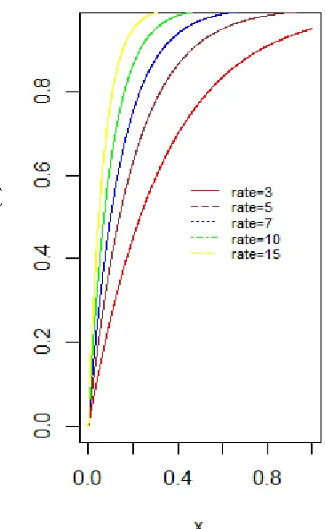
Figure 2: CDF curve of an Exponential Distribution at Different Values of Rate Parameter

2.0 MATERIALS AND METHODS 2.1 Prior Inormation

In Bayesian statistics, a prior probability information which is also known as prior distribution of an uncertain quantity is the probability distribution that would express one’s beliefs about this quantity before evidence is considered. The most important part of a Bayesian estimation is the specification of a prior distribution.

Although, at times priors are chosen according to one’s subjective knowledge and belief that is why Bayesian approach is sometimes called a subjective approach [4]. In this research work two types of prior information will be adopted namely; non-informative prior distribution (such as extension of Jeffrey’s prior distribution) and informative prior distribution (such as Gamma prior distribution, Gamma-Chi-square prior distribution, Gamma – Exponential prior distribution and Chi-square-Exponential prior distribution).

2.1.1 Extension of the Jefferey’s Prior:

The prior proposed by [3], [11] and [13], known as extension of Jeffrey’s prior is given by

𝑔(𝛾) ∝ [𝐼(𝛾)]𝑘_{; 𝑘 ∈ ℛ}+ ₍₃₎

Where 𝐼(𝛾) = −𝑛𝐸 [𝜕2

𝜕𝛾2𝑙𝑜𝑔𝑓(𝑥; 𝛾)] is known as Fisher’s information matrix. Therefore 𝐼(𝛾) for Exponential distribution will be

𝐼(𝛾) = −𝑛 [𝜕2

𝜕𝛾2{ln 𝛾 − 𝛾𝑥}] (4) Thus, the resulting extension of Jeffrey’s prior will be

𝑔1(𝛾) ∝ ( 1 𝛾2)

𝑘

(5)

Remark 1: if 𝑘 = 1

2, we will have Jeffrey’s prior

𝑔11(𝛾) ∝ 1_𝛾 (6) Remark 2: if 𝑘 = 3

2, we will have Hartigan’s prior

𝑔₁₂(𝛾) ∝ _𝛾13 (7) Remark 3: if 𝑘 = 0, we will have U (0, k=1

𝑝) prior

𝑔₁₃(𝛾) ∝ 1 (8) 2.1.2 The Gamma Prior

The single prior distribution of 𝛾 is a Gamma distribution with hyper parameters 𝛼1 and 𝛽1 is

𝑔2(𝛾) = 𝛽₁𝛼1 𝚪(𝛼1)𝛾

𝛼1−1_𝑒−𝛽1𝛾_;𝛼₁> 0 , 𝛽

ISSN 2250-3153

Assume that the prior distribution of 𝛾 is a Gamma distribution with hyper parameters 𝛼2 and 𝛽2 as

𝑔31(𝛾) = 𝛽2𝛼2 𝚪(𝛼2)𝛾

𝛼2−1_𝑒−𝛽2𝛾_{; 𝛼}

2> 0 , 𝛽2> 0 (10)

The second prior assumed is a Chi-square distribution with hyper parameter 𝜓1 given by

𝑔₃₂(𝛾) = 1

2 𝜓1

2 Γ(𝜓12 )

𝛾𝜓12−1𝑒− 𝛾

2 ; 𝜓₁> 0, 𝛾 > 0 ₍₁₁₎ [1] defined the double prior for 𝛾 by combining the two priors in (10) and (11) as:

𝑔3(𝛾) ∝ 𝑔31(𝛾)𝑔32(𝛾)

𝑔3(𝛾) ∝ 𝛾𝛼2+ 𝜓1

2−2𝑒−𝛾( 1

2+𝛽2) ₍₁₂₎ 2.1.4 Gamma - Exponential distribution

The double prior for 𝛾 is defined to be a Gamma distribution with hyper parameters (𝛼₃, 𝛽₃)and an exponentialdistribution with hyper parameter 𝛿1as

𝑔₄₁(𝛾) =𝛽3𝛼3 𝚪(𝛼3)𝛾

𝛼3−1_𝑒−𝛽3𝛾_;𝛼₃> 0 , 𝛽

3> 0 (13)

𝑔₄₂(𝛾) = 𝛿1𝑒𝛿1𝛾; 𝛿1> 0 (14)

[1] defined the double prior for 𝛾 by combining the two priors in (13) and (14) as:

𝑔₄∝ 𝑝₃(𝛾)𝑝₄(𝛾)

𝑔₄∝ 𝛾𝛼3−1_𝑒−𝛾(𝛿1+𝛽3) ₍₁₅₎ 2.1.5 Chi-Square-Exponential Prior

The double prior for 𝛾 is defined to be a Gammadistribution with hyper parameters 𝜓₂and an exponentialdistribution with hyper parameter 𝛿2as

𝑔₅₁(𝛾) = 1

2 𝜓2

2Γ(𝜓22)

𝛾𝜓22−1𝑒− 𝛾

2 ; 𝜓₂> 0, 𝛾 > 0 ₍₁₆₎

𝑔₅₂(𝛾) = 𝛿₂𝑒𝛿2𝛾_{; 𝛿}

2> 0 (17) [1] defined a double prior for 𝛾 by combining the two priors in (16) and (17) as:

𝑔₅∝ 𝛾𝜓22−1𝑒−𝛾( 1

2+𝛿2) ₍₁₈₎

2.1 Loss Function

The concept of loss function is as old as Laplace and wad reintroduced in statistics by Abraham Wald in the middle of 20th Century. Sound statistical practice requires selecting an estimator consistent with the actual acceptable variation experienced in the context of a particular applied problem. In this paper we considered the use of Al-Bayyati’s loss function for better comparison of Bayes’ estimators.

2.1.1 Al-Bayyati’s Loss Function

The Al-Bayyati’s loss function was stated by [7] as

𝑅_𝐴𝐿(𝛾̂, 𝛾) = 𝛾𝑐2_{(𝛾̂ − 𝛾)}2_{; 𝑐}

2∈ ℛ+ (19) Where 𝛾̂ is the estimated value of parameter 𝛾. 3. ESTIMATION

3.1 Maximum Likelihood Estimation

Let𝑥₁, 𝑥₂, ⋯ , 𝑥_𝑛 be a random sample size n from Exponential distribution. The maximum likelihood estimator 𝛾 of the

parameter 𝛾 which maximizes the likelihood function will be as follows [15] and [16]

𝐿(𝑥; 𝛾) = ∏ 𝑓(𝑥; 𝛾)

𝑛

𝑖=1

𝐿(𝑥; 𝛾) = 𝛾𝑛_𝑒−𝛾 ∑ 𝑥

The log-likelihood function for an Exponential distribution can be expressed as

log L(𝛾|x) = nlog𝛾 − 𝛾∑𝑥 (20) Now solving 𝜕

𝜕𝛾𝑙𝑜𝑔{𝐿(𝛾|𝑥)} = 0

𝛾̂ = (∑ 𝑥

𝑛) −1

(21) 3.2 Bayesian Estimation

To obtain Bayes estimators, we assume that𝛾 is a real valued random variable with probability density function 𝑔(𝛾). The posterior distribution of 𝛾 i. e, ℎ(𝛾|𝑥) is theconditional probability density function of𝛾 given the data. In this section weconsider Bayes estimation of the unknown parameter 𝛾 based on the above-mentioned priors and loss function.

3.2.1 Posterior Distribution of Unknown Parameter 𝜸 Using extension of the Jeffrey’s Prior

The posterior distribution for 𝛾 using extension of the Jeffrey’s prior

ℎ₁(γ|x) = 𝐿(𝑥|γ)𝑔1(γ) ∫ 𝐿(𝑥|γ)𝑔1(γ) ∂γ

∞ 0

ℎ1(γ|x) ∝

𝛾𝑛_𝑒− 𝛾 ∑ 𝑥₍1 𝛾2)

𝑘

∫ 𝛾𝑛_𝑒− 𝛾 ∑ 𝑥₍1 𝛾2)

𝑘

∂γ

∞ 0

𝑝(𝛾|𝑦) ∝ 𝛾𝑛−2𝑘_𝑒−𝛾 ∑ 𝑥

which is the density function of a Gamma distribution of

ℎ₁(γ|x) ∝ (∑ 𝑥)𝑛−2𝑘+1

Γ(𝑛−2𝑘+1)𝛾

𝑛−1_𝑒−𝛾 ∑ 𝑥 ₍₂₂₎ with parameters (n-2k+1 , ∑ 𝑥 ).

𝑀𝑒𝑎𝑛 = 𝐸(𝑋) = 𝑛 − 2𝑘 + 1 ∑ 𝑥

𝑉𝑎𝑟(𝑋) = 𝑛 − 2𝑘 + 1 ∑ 𝑥2

3.2.2 Posterior Distribution of Unknown Parameter 𝜸

Using Gamma Prior

The posterior distribution for 𝛾 using Gamma prior

ℎ₂(γ|x) = 𝐿(𝑥|γ)𝑔2(γ) ∫ 𝐿(𝑥|γ)𝑔2(γ) ∂γ

∞ 0

ℎ2(γ|x) ∝

𝛾𝑛_𝑒− 𝛾 ∑ 𝑥_𝛾𝛼₁−1_𝑒−𝛽₁𝛾

∫ 𝛾∞ 𝑛_𝑒− 𝛾 ∑ 𝑥_𝛾𝛼₁−1_𝑒−𝛽₁𝛾_∂γ 0

ℎ₂(γ|x) ∝ 𝛾𝑛+𝛼1−1_𝑒−𝛾(𝛽1+∑ 𝑥)

which is the density function of a Gamma distribution of

ℎ2(γ|x) =

(𝛽1+∑ 𝑥)𝑛+𝛼1 Γ(𝑛+𝛼1) 𝛾

ISSN 2250-3153

𝑀𝑒𝑎𝑛 = 𝐸(𝑥) = 𝑛 +𝛼1

𝛽₁+∑ 𝑥

𝑉𝑎𝑟(𝑥) = 𝑛 +𝛼1 ( 𝛽₁+∑ 𝑥)2

3.2.3 Posterior Distribution of Unknown Parameter 𝜸 Using Gamma-Chi-Square Prior

The posterior distribution for γ using Gamma-Chi-Square Prior

ℎ3(γ|x) =

𝐿(𝑥|γ)𝑔₃(γ) ∫ 𝐿(𝑥|γ)𝑔3(γ) ∂γ

∞ 0

ℎ₃(γ|x) ∝ 𝛾

𝑛_𝑒− 𝛾 ∑ 𝑥_𝛾𝛼2+𝜓1₂−2_𝑒−𝛾(1₂+𝛽2)

∫ 𝛾∞ 𝑛_𝑒− 𝛾 ∑ 𝑥_𝛾𝛼2+𝜓1₂−2_𝑒−𝛾(1₂+𝛽2)_∂γ 0

ℎ3(γ|x) ∝ 𝛾(𝛼2+ 𝜓1

2+𝑛−1)−1_𝑒−𝛾(𝛽1+∑ 𝑥+1₂) which is the density function of a Gamma distribution of

ℎ3(γ|x)

= (𝛽1+ ∑ 𝑥 +

1 2)

𝛼2+𝜓1₂+𝑛−1

Γ(𝛼2+ 𝜓1

2 + 𝑛 − 1)

𝛾(𝛼2+𝜓1₂+𝑛−1)−1_𝑒−𝛾(𝛽1+∑ 𝑥+1₂)

(24) With parameters (𝛼₂+𝜓1

2 + 𝑛 − 1, 𝛽1+ ∑ 𝑥 + 1 2)

𝑀𝑒𝑎𝑛 = 𝐸(𝑥) = 𝑛 + 𝛼2+

𝜓1 2 − 1

𝛽₂+∑ 𝑥 +1

2

𝑉𝑎𝑟(𝑥) =𝐧 + 𝛂𝟐+

𝛙𝟏 𝟐 − 𝟏

(𝛃_𝟐+∑ 𝐱 +𝟏_𝟐)𝟐

3.2.4 Posterior Distribution of Unknown Parameter 𝜸

Using Gamma-Exponential Prior

The posterior distribution for γ using Gamma-Exponential Prior

ℎ₄(γ|x) = 𝐿(𝑥|γ)𝑔4(γ) ∫ 𝐿(𝑥|γ)𝑔4(γ) ∂γ

∞ 0

ℎ₄(γ|x) ∝ 𝛾

𝑛_𝑒− 𝛾 ∑ 𝑥_𝛾𝛼3−1_𝑒−𝛾(𝛿1+𝛽3)

∫ 𝛾∞ 𝑛_𝑒− 𝛾 ∑ 𝑥_𝛾𝛼₃−1_𝑒−𝛾(𝛿1+𝛽3)∂γ 0

𝑝(𝛾|𝑥) ∝ 𝛾𝑛+𝛼3−1_𝑒−𝛾(𝛿1+𝛽3+∑ 𝑥)

which is the density function of a Gamma distribution of

𝑝(𝛾|𝑋) = (𝛿1+ 𝛽3+ ∑ 𝑥)

𝑛+𝛼3

Γ(𝑛 + 𝛼₃) 𝛾

𝑛+𝛼₃−1_𝑒−𝛾(𝛿1+𝛽3+∑ 𝑥) (25) With parameters (𝑛 + 𝛼₃,𝛿₁+ 𝛽₃+∑𝑥)

𝑀𝑒𝑎𝑛 = 𝐸(𝑋) = 𝑛 + 𝛼3 𝛿₁+ 𝛽₃+ ∑ 𝑥

𝑉𝑎𝑟(𝑋) = 𝑛 + 𝛼3 ( 𝛿1+ 𝛽3+ ∑ 𝑥)2

3.2.5 Posterior Distribution of Unknown Parameter 𝜸

Using Chi-Square-Exponential Prior

ℎ₅(γ|x) = 𝐿(𝑥|γ)𝑔5(γ) ∫ 𝐿(𝑥|γ)𝑔5(γ) ∂γ

∞ 0

ℎ5(γ|x) ∝

𝛾𝑛_𝑒− 𝛾 ∑ 𝑥_𝛾𝜓2₂−1_𝑒−𝛾(1₂+𝛿2)

∫ 𝛾𝑛_𝑒− 𝛾 ∑ 𝑥_𝛾𝜓22−1𝑒−𝛾( 1 2+𝛿2)∂γ ∞

0

ℎ₅(γ|x) ∝ 𝛾(𝑛+𝜓22−1)𝑒−𝛾(𝛿2+∑ 𝑥+ 1 2) which is the density function of a Gamma distribution of

ℎ₅(γ|x) = (𝛿2+ ∑ 𝑥 +

1 2)

𝑛+𝜓2₂

Γ(𝑛 +𝜓2 2)

𝛾(𝜓22+𝑛−1)𝑒−𝛾(𝛿2+∑ 𝑥+ 1 2)

(26) With parameters (𝑛 +𝜓2

2 , 𝛿2+ ∑ 𝑥 + 1 2)

𝑀𝑒𝑎𝑛 = 𝐸(𝑥) = 𝑛 +

𝜓2 2

𝛿2+ ∑ 𝑥 + 1 2

𝑉𝑎𝑟(𝑥) = 𝑛 +

𝜓2 2

(𝛿2+ ∑ 𝑥 +1₂) 2

3.3 Bayes’ Estimator Under Al-Bayyati’s Loss Function The risk function under Al-Bayyati’s loss function can be define is

𝑅(𝐴𝐿,𝐸𝐽)(𝛾̂) = ∫ 𝛾𝑐2(𝛾̂ − 𝛾)2ℎ𝑖(𝛾|𝑥)𝜕𝛾 ∞

0 (27)

3.3.1 Extension of Jeffrey’s Prior

The risk function under Al-Bayyati’s loss function using extension of Jeffrey’s prior is given by

𝑅_{(𝐴𝐿,𝐸𝐽)}(𝛾̂) = ∫ 𝛾𝑐2_{(𝛾̂ − 𝛾)}2_ℎ

1(𝛾|𝑥)𝜕𝛾 ∞

0

𝑅_{(𝐴𝐿,𝐸𝐽)}(𝛾̂) = ∫ 𝛾𝑐2_{(𝛾̂ − 𝛾)}2 (∑ 𝑥) 𝑛−2𝑘+1

Γ(𝑛−2𝑘+1)𝛾

𝑛−1_𝑒−𝛾 ∑ 𝑥_𝜕𝛾 ∞

0 (28)

𝑅_{(𝐴𝐿,𝐸𝐽)}(𝛾̂) = 𝛾̂

2_{Γ(𝑛 − 2𝑘 + 𝑐} 2+ 1)

Γ(𝑛 − 2𝑘 + 1)(∑ 𝑥)𝑐2+1

− 2𝛾̂Γ(𝑛 − 2𝑘 + 𝑐2+ 2) Γ(𝑛 − 2𝑘 + 1)(∑ 𝑥)𝑐2+1

+ Γ(𝑛 − 2𝑘 + 𝑐2+ 3) Γ(𝑛 − 2𝑘 + 1)(∑ 𝑥)𝑐2+2

Now, solving 𝑅(𝐴𝐿,𝐸𝐽)_𝜕𝛾̂ (𝛾̂)= 0 for 𝛾̂ yield the required Bayes’ estimator under the assumed combination of loss function and prior distribution in given by

𝛾̂_{(𝐴𝐿,𝐸𝐽)}= 𝑛−2𝑘+𝑐2+1

∑ 𝑥 (29)

3.3.2 Gamma Prior Distribution

The risk function under Al-Bayyati’s loss function using extension of Gamma prior is given by

𝑅(𝐴𝐿,𝐺𝑃)(𝛾̂) = ∫ 𝛾𝑐2(𝛾̂ − 𝛾)2ℎ2(𝛾|𝑥)𝜕𝛾 ∞

0

𝑅(𝐴𝐿,𝐺𝑃)(𝛾̂) = ∫ 𝛾𝑐2(𝛾̂ ∞

0

− 𝛾)2(𝛽1+ ∑ 𝑥)𝑛+𝛼1

Γ(𝑛 + 𝛼₁) 𝛾

ISSN 2250-3153

(30)

𝑅_{(𝐴𝐿,𝐺𝑃)}(𝛾̂) = 𝛾̂

2_{Γ(𝑛 + 𝛼} 1+ 𝑐2)

Γ(𝑛 + 𝛼₁)(∑ 𝑥 + 𝛽₁)𝑐2

− 2𝛾̂Γ(𝑛 + 𝛼1+ 𝑐2+ 1) Γ(𝑛 + 𝛼₁)(∑ 𝑥 + 𝛽₁)𝑐2+1

+ Γ(𝑛 + 𝛼1+ 𝑐2+ 2) Γ(𝑛 + 𝛼₁)(∑ 𝑥 + 𝛽₁)𝑐2+2

Now, solving 𝑅(𝐴𝐿,𝐺𝑃)_𝜕𝛾̂ (𝛾̂)= 0 for 𝛾̂ yield the required bayes estimator under the assumed combination of loss function and prior distribution in given by

𝛾̂_{(𝐴𝐿,𝐺𝑃)}= 𝑛+𝛼1+𝑐2

∑ 𝑥+𝛽1 (31)

3.3.3 Gamma- Chi-Square Prior Distribution

The risk function under Al-Bayyati’s loss function using extension of Gamma- Chi-square prior is given by

𝑅_{(𝐴𝐿,𝐺𝐶)}(𝛾̂) = ∫ 𝛾𝑐2_{(𝛾̂ − 𝛾)}2_ℎ

3(𝛾|𝑥)𝜕𝛾 ∞

0

𝑅(𝐴𝐿,𝐺𝐶)(𝛾̂) = ∫ 𝛾₀∞ 𝑐2(𝛾̂ −

𝛾)2(𝛽1+∑ 𝑥+1₂)

𝛼2+𝜓1_{2 +𝑛−1}

Γ(𝛼2+𝜓1₂+𝑛−1)

𝛾(𝛼2+𝜓1₂+𝑛−1)−1_𝑒−𝛾(𝛽1+∑ 𝑥+1₂)_𝜕𝛾 (32)

𝑅_{(𝐴𝐿,𝐺𝐶)}(𝛾̂) = 𝛾̂

2_{Γ (𝑛 + 𝛼} 2+

𝜓1

2 + 𝑐2− 1)

Γ (𝑛 + 𝛼₂+𝜓1

2 − 1) (∑ 𝑥 + 1 2+ 𝛽1)

𝑐2

− 2𝛾̂Γ (𝑛 + 𝛼2+

𝜓1 2 + 𝑐2)

Γ (𝑛 + 𝛼2+ 𝜓1

2 − 1) (∑ 𝑥 + 1 2+ 𝛽1)

𝑐2+1

+ Γ (𝑛 + 𝛼2+

𝜓1 2 + 𝑐2)

Γ (𝑛 + 𝛼₂+𝜓1

2 − 1) (∑ 𝑥 + 1 2+ 𝛽1)

𝑐2+2

Now, solving 𝑅(𝐴𝐿,𝐺𝐶)(𝛾̂)

𝜕𝛾̂ = 0 for 𝛾̂ yield the required bayes estimator under the assumed combination of loss function and prior distribution in given by

𝛾̂(𝐴𝐿,𝐺𝐶)=

𝑛+𝛼2+𝜓1₂+𝑐2−1

∑ 𝑥+1₂+𝛽1 (33) 3.3.4 Gamma- Exponential Prior Distribution

The risk function under Al-Bayyati’s loss function using extension of Gamma- Exponential prior is given by

𝑅(𝐴𝐿,𝐺𝐸)(𝛾̂) = ∫ 𝛾𝑐2(𝛾̂ − 𝛾)2ℎ3(𝛾|𝑥)𝜕𝛾 ∞

0

𝑅_{(𝐴𝐿,𝐺𝐸)}(𝛾̂) = ∫ 𝛾∞ 𝑐2_{(𝛾̂ −} 0

𝛾)2 (𝛿1+𝛽3+∑ 𝑥)𝑛+𝛼3 Γ(𝑛+𝛼3) 𝛾

𝑛+𝛼3−1_𝑒−𝛾(𝛿1+𝛽3+∑ 𝑥)_𝜕𝛾 (34)

𝑅_{(𝐴𝐿,𝐺𝐶)}(𝛾̂) = 𝛾̂

2_{Γ(𝑛 + 𝛼}

3+ 𝑐2+ 2)

Γ(𝑛 + 𝛼₃+ 2)(∑ 𝑥 + 𝛽₃+ 𝛿₁)𝑐2

− 2𝛾̂Γ(𝑛 + 𝛼3+ 𝑐2+ 3) Γ(𝑛 + 𝛼₃+ 2)(∑ 𝑥 + 𝛽₃+ 𝛿₁)𝑐2+1

+ Γ(𝑛 + 𝛼3+ 𝑐2+ 4) Γ(𝑛 + 𝛼₃+ 2)(∑ 𝑥 + 𝛽₃+ 𝛿₁)𝑐2+2 Now, solving 𝑅(𝐴𝐿,𝐺𝐸)(𝛾̂)

𝜕𝛾̂ = 0 for 𝛾̂ yield the required bayes estimator under the assumed combination of loss function and prior distribution in given by

𝛾̂(𝐴𝐿,𝐺𝐸)= 𝑛+𝛼_{∑ 𝑥+𝛽}3+𝑐2+2

3+𝛿1 (35)

3.3.5 Chi-Square-Exponential Prior Distribution

The risk function under Al-Bayyati’s loss function using extension of Chi-square-Exponential prior is given by

𝑅(𝐴𝐿,𝐶𝐸)(𝛾̂) = ∫ 𝛾𝑐2(𝛾̂ − 𝛾)2ℎ3(𝛾|𝑥)𝜕𝛾 ∞

0

𝑅(𝐴𝐿,𝐶𝐸)(𝛾̂) = ∫ 𝛾𝑐2(𝛾̂ − ∞

0

𝛾)2(𝛿2+∑ 𝑥+ 1 2)

𝑛+𝜓2₂

Γ(𝑛+𝜓2₂) 𝛾

(𝜓2₂+𝑛−1)_𝑒−𝛾(𝛿2+∑ 𝑥+1₂)_𝜕𝛾 (36)

𝑅(𝐴𝐿,𝐶𝐸)(𝛾̂) =

𝛾̂2_{Γ (}𝜓2

2 + 𝑛 + 𝑐2)

Γ (𝜓2

2 + 𝑛) (𝛿2+ ∑ 𝑥 + 1 2)

𝑐2

− 2𝛾̂Γ (𝑛

𝜓2

2 + 𝑛 + 𝑐2+ 1)

Γ (𝜓2

2 + 𝑛) (𝛿2+ ∑ 𝑥 + 1 2)

𝑐2+1

+ Γ (

𝜓2

2 + 𝑛 + 𝑐2+ 2)

Γ (𝜓2

2 + 𝑛) (𝛿2+ ∑ 𝑥 + 1 2)

𝑐2+2

Now, solving 𝑅(𝐴𝐿,𝐶𝐸)(𝛾̂)

𝜕𝛾̂ = 0 for 𝛾̂ yield the required bayes estimator under the assumed combination of loss function and prior distribution in given by

𝛾̂(𝐴𝐿,𝐶𝐸)= 𝜓2

2+𝑛+𝑐2

𝛿2+∑ 𝑥+1₂ (37)

Now, on summarizing the above Bayes’ estimators and their special cases, we can have the following table of estimators

Table 1: Bayes’ Estimators under Al-Bayyati’s loss function and Different Prior Distributions

Prior Estimator

Extension of

Jeffrey’s 𝛾̂(𝐴𝐿,𝐸𝐽)=

𝑛 − 2𝑘 + 𝑐2+ 1

∑ 𝑥

Hartigan’s

𝛾̂(𝐴𝐿,𝐸𝐽)=

𝑛 − 2 + 𝑐2

∑ 𝑥

Jeffrey’s

𝛾̂(𝐴𝐿,𝐸𝐽)=

𝑛 + 𝑐2

ISSN 2250-3153

Uniform

𝛾̂(𝐴𝐿,𝐸𝐽)=

𝑛 + 𝑐2+ 1

∑ 𝑥

Gamma _𝛾̂

(𝐴𝐿,𝐺𝑃)=

𝑛 + 𝛼1+ 𝑐2

∑ 𝑥 + 𝛽₁

Gamma-Chi-squares 𝛾̂_{(𝐴𝐿,𝐺𝐶)}= 𝑛 + 𝛼2+

𝜓1

2 + 𝑐2− 1

∑ 𝑥 +1

2+ 𝛽1

Gamma-Exponential 𝛾̂(𝐴𝐿,𝐺𝐸)=

𝑛 + 𝛼3+ 𝑐2+ 2

∑ 𝑥 + 𝛽₃+ 𝛿1

Chi-Squares-Exponential 𝛾̂(𝐴𝐿,𝐶𝐸)= 𝜓₂

2 + 𝑛 + 𝑐2

𝛿2+ ∑ 𝑥 + 1 2 Note: Subscript in the form ordered pair in each estimator represents the combination of Al-Bayyati’s loss function and prior distribution used in the derivation of Bayes’ estimator. First element of the ordered pair represents Al-Bayyati’s loss function whereas the second element represent prior distribution.

4.0 SIMULATION STUDY OF AN EXPONENTIAL DISTRIBUTION

In the simulation study, data sets of size n = 50, 100, 200 and 500 have been generated from Exponential distribution with parameter k taking the values 0, 0.5, 1 and 1.5. Whereas, values of another hyper-parameter 𝑐₂ are considered to be 1 and 3. We also set 𝛼1= 1.5, 3 , 𝛼2= 1, 2, 𝛼3= 1, 2 , 𝛽1=

1, 5, 𝛽₂= 1.5, 3 , 𝛽₃= 1.5, 3, 𝜓₁= 0.5, 1, 𝜓₂= 1.5, 3 , 𝛿₁= 0.5 , 1 and 𝛿₂= 1, 2 . We carried out simulation using R programming language.

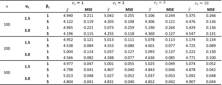
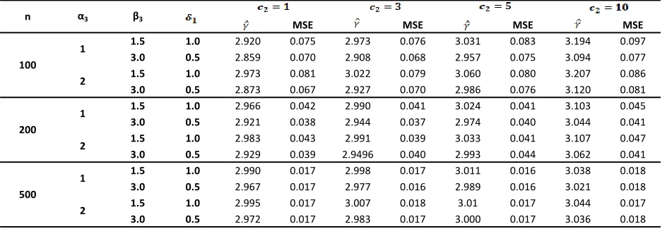
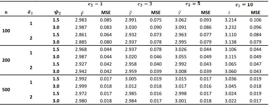
The results presented in Tables 2 and 3 displayed the expected an MSE’s for estimating the rate parameter 𝛾 under the Extension Jeffrey prior distribution. The results in Tables 4 and 5 displayed the expected and MSE’s for estimating the

rate parameter 𝛾 under the Gamma prior distribution. Tables 6 and 7 displayed the expected and MSE’s for estimating the rate parameter 𝛾 under the Gamma-Chi-squares prior distribution. Tables 8 and 9 displayed the expected and MSE’s for estimating the rate parameter 𝛾 under the Gamma-Exponential prior distribution. Tables 10 and 11 displayed the expected and MSE’s for estimating the rate parameter

𝛾 under the Chi-squares-Exponential prior distribution. It was observed that on considering the Hartigan’s prior (k =1.5), usually parameter gets under estimated and starts overestimating it as 𝑐2 increases from 1 to 10. The behaviour

of Bayesian estimates for all infomative prior distribuitons have better behaviour than other estimates when compared with estimates of non-informative prior distribution for different sample sizes and various rate parameters. Finally, for all parameter values, as the sample size increases the MSE keeps reducing.

Table 2: Bayes’ Estimates of Estimators along with their Mean Square Errors under Extension of Jeffrey prior distribution when γ=3

MSE MSE MSE MSE

0.0 3.086 0.099 3.141 0.099 3.216 0.103 3.365 0.119

0.5 3.365 0.119 3.058 0.095 3.174 0.101 3.331 0.109

1.0 3.005 0.084 3.099 0.099 3.138 0.103 3.300 0.108

1.5 2.989 0.095 3.066 0.095 3.123 0.095 3.264 0.106

0.0 3.056 0.048 3.090 0.045 3.101 0.045 3.182 0.054

0.5 3.023 0.047 3.065 0.046 3.094 0.048 3.169 0.046

1.0 3.020 0.046 3.036 0.055 3.073 0.048 3.510 0.049

1.5 2.999 0.046 3.042 0.048 3.062 0.049 3.148 0.049

0.0 3.014 0.018 3.031 0.019 3.035 0.02 3.067 0.018

0.5 3.013 0.020 3.030 0.020 3.035 0.017 '3.070 0.020

1.0 3.002 0.019 3.018 0.017 3.031 0.018 3.056 0.018

1.5 3.003 0.018 3.016 0.018 3.027 0.018 3.054 0.019 100

n

200

ISSN 2250-3153

Table 3: Bayes’ Estimates of Estimators along with their Mean Square Errors under Extension of Jeffrey prior distribution when γ=5

MSE MSE MSE MSE

0.0 5.118 0.265 5.250 0.262 5.023 0.023 5.630 0.353

0.5 5.098 0.263 5.214 0.260 5.021 0.023 5.540 0.302

1.0 5.042 0.245 5.151 0.285 5.024 0.023 5.537 0.308

1.5 4.993 0.271 5.132 0.271 5.019 0.022 5.456 0.274

0.0 5.017 0.123 5.134 0.138 5.179 0.134 5.299 0.152

0.5 5.062 0.125 5.089 0.135 5.151 0.130 5.274 0.137

1.0 5.008 0.122 5.085 0.138 5.142 0.133 5.260 0.138

1.5 4.993 0.123 5.049 0.133 5.095 0.136 5.237 0.140

0.0 5.018 0.049 5.051 0.049 5.072 0.048 5.111 0.053

0.5 5.016 0.053 5.044 0.049 5.053 0.049 5.108 0.054

1.0 5.003 0.051 5.025 0.051 5.051 0.053 5.114 0.052

1.5 5.005 0.053 5.019 0.047 5.039 0.049 5.090 0.053 100

200

500 n

Table 4: Bayes’ Estimates of Estimators along with their Mean Square Errors under Gamma prior distribution when γ= 3

MSE MSE MSE MSE

1 3.015 0.083 3.066 0.087 3.119 0.099 3.275 0.102

5 2.702 0.056 2.746 0.058 2.798 0.058 2.927 0.068

1 3.037 0.085 3.110 0.087 3.170 0.093 3.137 0.100

5 2.748 0.056 2.785 0.059 2.837 0.066 2.966 0.066

1 3.005 0.045 3.024 0.047 3.056 0.047 3.140 0.045

5 2.835 0.034 2.873 0.036 2.906 0.038 2.967 0.038

1 3.032 0.043 3.059 0.046 3.085 0.047 3.155 0.046

5 2.866 0.034 2.877 0.034 2.918 0.038 2.981 0.042

1 3.015 0.016 3.010 0.018 3.028 0.018 3.057 0.018

5 2.934 0.017 2.941 0.017 2.958 0.017 2.980 0.016

1 3.015 0.018 3.025 0.018 3.033 0.018 3.075 0.019

5 2.942 0.016 2.946 0.016 2.969 0.017 2.997 0.017

200

1.5

3.0

500

1.5

3.0

n α1 β1

100

1.5

3.0

Table 5: Bayes’ Estimates of Estimators along with their Mean Square Errors under Gamma prior distribution when γ= 5

MSE MSE MSE MSE

1 4.940 0.211 5.042 0.255 5.106 0.244 5.375 0.266

5 4.122 0.119 4.203 0.108 4.306 0.121 4.476 0.136

1 4.965 0.221 5.073 0.259 5.190 0.264 5.429 0.136

5 4.196 0.115 4.255 0.118 4.360 0.127 4.547 0.131

1 4.952 0.121 5.013 0.111 5.078 0.113 5.174 0.134

5 4.538 0.084 4.553 0.080 4.601 0.077 4.725 0.089

1 5.004 0.114 5.037 0.127 5.093 0.137 5.222 0.130

5 4.566 0.082 4.588 0.077 4.636 0.085 4.771 0.100

1 4.977 0.047 5.001 0.055 5.025 0.049 5.074 0.052

5 4.798 0.041 4.807 0.040 4.843 0.046 4.878 0.042

1 5.013 0.048 5.027 0.052 5.037 0.053 5.092 0.048

5 4.804 0.041 4.831 0.040 4.852 0.042 4.907 0.044

200

1.5

3.0

500

1.5

3.0

n α1 β1

100

1.5

ISSN 2250-3153

Table 6: Bayes’ Estimates of Estimators along with their Mean Square Errors under Gamma – Chi-Squares prior distribution when γ= 3

MSE MSE MSE MSE

1.5 1.0 2.812 0.0704 2.880 0.081 2.933 0.078 3.082 0.092

3.0 0.5 2.700 0.059 2.761 0.065 2.815 0.033 2.946 0.071

1.5 1.0 2.811 0.076 2.879 0.085 2.920 0.078 3.077 0.082

3.0 0.5 2.688 0.061 2.740 0.062 2.785 0.064 2.928 0.068

1.5 1.0 2.902 0.042 2.951 0.041 2.964 0.042 3.035 0.048

3.0 0.5 2.839 0.037 2.789 0.036 2.887 0.038 2.980 0.043

1.5 1.0 2.893 0.038 2.925 0.038 2.961 0.042 3.023 0.042

3.0 0.5 2.838 0.035 2.881 0.037 2.897 0.040 2.972 0.039

1.5 1.0 2.957 0.017 2.974 0.019 2.993 0.017 3.025 0.018

3.0 0.5 2.931 0.016 2.946 0.017 2.956 0.018 2.987 0.017

1.5 1.0 2.969 0.018 2.979 0.017 2.985 0.019 3.014 0.019

3.0 0.5 2.930 0.017 2.946 0.016 2.960 0.017 2.993 0.017

n

100

200

500

α2 β2

1

2

1

2

1

2

Table 7: Bayes’ Estimates of Estimators along with their Mean Square Errors under Gamma – Chi-Squares prior distribution when γ= 5

MSE MSE MSE MSE

1.5 1.0 4.515 0.158 4.644 0.183 4.745 0.208 4.940 0.019

3.0 0.5 4.217 0.117 4.324 0.138 4.397 0.147 4.612 0.148

1.5 1.0 4.507 0.168 4.626 0.186 4.714 0.191 4.928 0.205

3.0 0.5 4.208 0.129 4.322 0.127 4.39 0.13 4.600 0.152

1.5 1.0 4.753 0.108 4.805 0.097 4.864 0.116 4.972 0.110

3.0 0.5 4.612 0.088 4.630 0.096 4.700 0.093 4.808 0.099

1.5 1.0 4.739 0.102 4.788 0.109 4.823 0.106 4.961 0.111

3.0 0.5 4.573 0.090 4.635 0.096 4.691 0.098 4.790 0.097

1.5 1.0 4.895 0.046 4.937 0.045 4.928 0.045 4.978 0.047

3.0 0.5 4.820 0.046 4.847 0.046 4.868 0.045 4.919 0.044

1.5 1.0 4.912 0.048 4.917 0.047 4.931 0.046 4.990 0.051

3.0 0.5 4.830 0.044 4.845 0.043 4.876 0.043 4.913 0.046

n

100

200

500

2 1

2

1

2

1

α2 β2

Table 8: Bayes’ Estimates of Estimators along with their Mean Square Errors under Gamma – Exponential prior distribution when γ=3

MSE MSE MSE MSE

1.5 1.0 2.920 0.075 2.973 0.076 3.031 0.083 3.194 0.097

3.0 0.5 2.859 0.070 2.908 0.068 2.957 0.075 3.094 0.077

1.5 1.0 2.973 0.081 3.022 0.079 3.060 0.080 3.207 0.086

3.0 0.5 2.873 0.067 2.927 0.070 2.986 0.076 3.120 0.081

1.5 1.0 2.966 0.042 2.990 0.041 3.024 0.041 3.103 0.045

3.0 0.5 2.921 0.038 2.944 0.037 2.974 0.040 3.044 0.041

1.5 1.0 2.983 0.043 2.991 0.039 3.033 0.041 3.107 0.047

3.0 0.5 2.929 0.039 2.9496 0.040 2.993 0.044 3.062 0.041

1.5 1.0 2.990 0.017 2.998 0.017 3.011 0.016 3.038 0.018

3.0 0.5 2.967 0.017 2.977 0.016 2.989 0.016 3.021 0.018

1.5 1.0 2.995 0.017 3.007 0.018 3.01 0.017 3.044 0.017

3.0 0.5 2.972 0.017 2.983 0.017 3.000 0.017 3.036 0.018

n

100

200

500

2 1

2

1

2

1

ISSN 2250-3153

Table 9: Bayes’ Estimates of Estimators along with their Mean Square Errors under Gamma – Exponential prior distribution when γ= 5

MSE MSE MSE MSE

1.5 1.0 4.652 0.178 4.763 0.201 4.829 0.183 5.082 0.198

3.0 0.5 4.428 0.144 4.543 0.16 4.622 0.154 4.817 0.157

1.5 1.0 4.689 0.169 4.777 0.171 4.883 0.184 5.128 0.214

3.0 0.5 4.51 0.156 4.601 0.154 4.666 0.149 4.890 0.799

1.5 1.0 4.819 0.097 4.873 0.103 4.914 0.107 5.030 0.100

3.0 0.5 4.714 0.097 4.765 0.09 4.797 0.097 4.917 0.099

1.5 1.0 4.854 0.105 4.906 0.113 4.924 0.105 5.070 0.119

3.0 0.5 4.737 0.096 4.785 0.099 4.817 0.099 4.932 0.103

1.5 1.0 4.934 0.051 4.935 0.046 4.970 0.051 5.011 0.046

3.0 0.5 4.885 0.046 4.912 0.045 4.913 0.049 4.966 0.045

1.5 1.0 4.939 0.048 4.950 0.046 4.969 0.049 5.025 0.045

3.0 0.5 4.874 0.045 4.908 0.041 4.932 0.043 4.969 0.042

500

1

2 100

1

2

200

1

2

n α3 β3

Table 10: Bayes’ Estimates of Estimators along with their Mean Square Errors under Chi-squares – Exponential prior distribution when γ=3

MSE MSE MSE MSE

1.5 2.983 0.085 2.991 0.075 3.062 0.093 3.214 0.106

3.0 2.987 0.083 3.030 0.090 3.091 0.086 3.232 0.096

1.5 2.861 0.064 2.932 0.073 2.963 0.077 3.110 0.084

3.0 2.885 0.080 2.937 0.078 2.995 0.079 3.138 0.079

1.5 2.968 0.044 2.937 0.078 3.026 0.044 3.106 0.044

3.0 2.987 0.044 3.020 0.046 3.055 0.049 3.115 0.049

1.5 2.927 0.042 2.958 0.040 2.992 0.043 3.065 0.047

3.0 2.942 0.042 2.959 0.039 3.008 0.039 3.060 0.043

1.5 2.992 0.017 3.005 0.019 3.015 0.017 3.036 0.019

3.0 2.999 0.018 3.012 0.018 3.017 0.016 3.045 0.018

1.5 2.972 0.017 2.985 0.016 2.998 0.017 3.024 0.019

3.0 2.980 0.018 2.984 0.017 3.001 0.018 3.022 0.017

500

1

2 100

1

2

200

1

ISSN 2250-3153

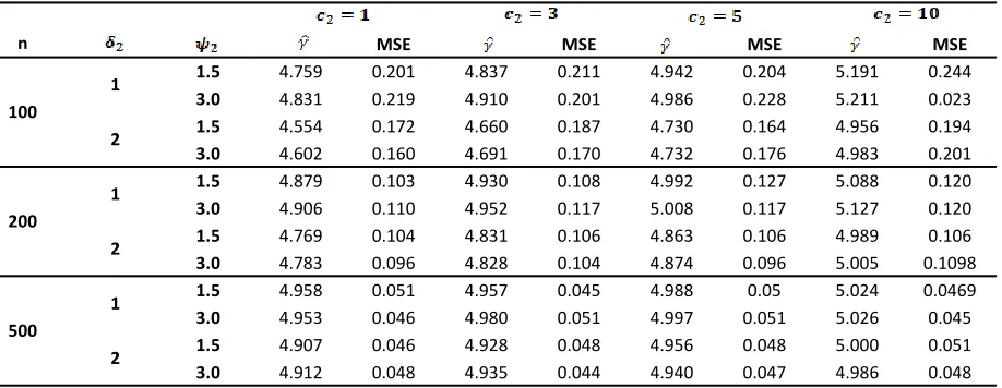
5.0 CONCLUSION

This research work emphasized on the importance of Bayesian approximation using Al-Bayyati’s loss function approach. Based on the results presented in Tables 2-11, we see that all the estimated values of the parameters are close to the true values of parameters in Exponential distribution. Bayesian estimates under informative prior distributions proves to be better than the estimates under the non-informative prior distributions proves to be efficient with minimum mean square error.

We conclude that the MSEs based on different prior distributions decreases as the sample size increases. It proves that the obtained estimates for the rate parameter are consistent. We also deduced that the performance of Bayesian estimates under informative prior distributions is better than non-informative prior.

ACKNOWLEDGMENT

The authors were grateful to the anonymous reviewers whose comments and suggestions were valuable to improve the exposition of the paper.

REFERENCES

[1] Adegoke T. M, Adegoke G. K, Yahya A. M., Uthman K.T. and Odigie A. D. (2018). Bayesian Posterior Estimates of an Exponential Distribution, 2nd _{International Conference} of the Nigeria Statistical Society, 8th _{– 9}th _{April, 2018:} University of Calabar, Cross River State, Nigeria.

[2] Al-Bayyatis H. N. (2002). Comparing Methods of estimating Webull Failure Models Using Simulation

(Ph.D. Thesis College of Administration and Economic, Baghdad Univ., Iraq).

[3] Al-Kutubi, H. S. (2005). On comparison estimation procedures for parameter and survival function exponential distribution using simulation. Ph.D. Thesis, Baghdad University, Iraq.

[4] Dar A. A, Ahmed A., and Reshi J. A. (2017). Bayesian Analysis of Maxwell-Boltzmann Distribution Under Different Loss Functions and Prior Distribution, Pakistan Journal of Statistics, 33(6), 419-440.

[5] Davis D.J (1952). An analysis of some failure data. Journal of American Statistical Association 47(258): 113-150.

[6] Elfessi, A. and Reineke, D. M. (2001). Bayesian look at classical estimation: the exponential distribution. Journal of Statistics Education, 9(1).

[7] Epstein, B. Sobel M (1953), Life testing. Journal of American Statistical Association 48(263): 486-502. Table 11: Bayes’ Estimates of Estimators along with their Mean Square Errors under Chi-squares – Exponential prior

distribution when γ=5

MSE MSE MSE MSE

1.5 4.759 0.201 4.837 0.211 4.942 0.204 5.191 0.244

3.0 4.831 0.219 4.910 0.201 4.986 0.228 5.211 0.023

1.5 4.554 0.172 4.660 0.187 4.730 0.164 4.956 0.194

3.0 4.602 0.160 4.691 0.170 4.732 0.176 4.983 0.201

1.5 4.879 0.103 4.930 0.108 4.992 0.127 5.088 0.120

3.0 4.906 0.110 4.952 0.117 5.008 0.117 5.127 0.120

1.5 4.769 0.104 4.831 0.106 4.863 0.106 4.989 0.106

3.0 4.783 0.096 4.828 0.104 4.874 0.096 5.005 0.1098

1.5 4.958 0.051 4.957 0.045 4.988 0.05 5.024 0.0469

3.0 4.953 0.046 4.980 0.051 4.997 0.051 5.026 0.045

1.5 4.907 0.046 4.928 0.048 4.956 0.048 5.000 0.051

3.0 4.912 0.048 4.935 0.044 4.940 0.047 4.986 0.048

500

1

2 100

1

2

200

1

ISSN 2250-3153

[8] Epstein, B. and Sobcl, M. (1984). Soethorems to life resting from an exponential distribution, Annals of Mathematical Statistics, 25.

[9] Epstein, B. (1958). The exponential distribution and its role in Life –testing. Industrial Quality Control 15: 2-7. [10] Feil P. and Zelen, M. (1965), Estimation of exponential

survival probabilities with concomitant information. Biometrics 21(4): 826-838.

[11] Al-Nasir, A. M. and Al-Kutunbi, H. S. (2006). Extension of Jeffery prior information. Iraq Journal of Statistical Science, 9:1-14.

[12] Ahmed A. A., Khan A.A., Ahmed S.P. (2007). Bayesian Analysis of Exponential Distribution on S-PLUS and R Software. Sri Lankan Journal of Applied Statistics, 8:95-109.

[13] SaimaNaqash, S. P. Ahmed and A. Ahmed (2015). Bayesian Analysis of Generalized Gamma Distribution. J. Stat. Appl. Pro. 4 (3): 499 -512

[14] Ahmed S.P. Ahmed, A. Khan A.A (2011). Bayesian Analysis of Gamma Distribution Using SPLUS and R-software. Asian J. Math., 4: 224-244

[15] Hogg, R.V., McKean, J.W. and Craig, A.T. (2014). Introduction to Mathematical Statistics, (7th _{ed.), Pearson} Education Publication.