WASTE COLLECTION VEHICLE ROUTING PROBLEM
BENCHMARK DATASETS AND CASE STUDIES: A REVIEW
1
ZANARIAH IDRUS, 2KU RUHANA KU-MAHAMUD, 3AIDA MAUZIAH BENJAMIN
1
Faculty of Computer & Mathematical Sciences, Universiti Teknologi MARA, Merbok, Kedah, Malaysia 2
School of Computing, College of Arts & Sciences, Universiti Utara Malaysia, Kedah, Malaysia 3
School of Quantitative Sciences, College of Arts & Sciences, Universiti Utara Malaysia, Kedah, Malaysia
E-mail: [email protected], [email protected], [email protected]
ABSTRACT
Waste collection vehicle routing problem (WCVRP) is one of the most studied areas and has received high interest from the modern society today. This corresponds to the cost efficiency, population growth, and environmental concerns. The growth of the WCVRP awareness is the result of continuous supports from government and private organizations. This paper reviews several established benchmark datasets and successful real-life case studies. Respectively billions of dollars have been saved from the operational costs. The current trend for benchmark datasets presented and case studies are accordingly grouped by countries and continents, thus revealing the need for WCVRP. Investigation on objectives, constraints and algorithms are also discussed. Results showed the increased interest of researchers in using benchmark datasets as well as the case studies and some of the constraints that should be considered in WCVRP. It also suggested that environmental or quality of service issues can be integrated into the common objectives of minimizing cost and distance travelled. Methods used in WCVRP are exact methods and approximate methods. Results showed that approximate methods have the capability in providing good results for large-scale data. Conclusively, this study analyzes the gap and provides recommendations for researches.
Keywords: Waste Management, Approximate & Exact Algorithms, Benchmark Datasets, Vehicle Routing
Problem
1. INTRODUCTION
Waste collection vehicle routing problem (WCVRP) is an important and emerging research topic as it is vital from economic and environmental perspective due to the increase amount of generated waste and the complexity of the products.
Waste is defined as by-products or end products of the production and consumption process and can be classified as residential, commercial, and industrial or roll-on-roll-off [1]. Residential waste generally involves waste collection from residential communities and private homes, in which vehicles move along the streets to collect garbage from small bins. The frequency of the waste collection service depends on the climate, geography, and service charge. Commercial waste is waste collected from malls, restaurants, and small office buildings, which usually have bigger size of bins. It is fairly static and has a consistent frequency of service. Industrial waste, on the other hand, involves garbage collection from construction sites, downtown area,
and large shopping malls. Industrial and commercial waste collections do not only differ by the size of containers, but also by their route. Industrial waste vehicles deliver an additional empty container at the customer’s location, pick up the full container, travel to a disposal facility, and empty the container [2].
ISSN: 1992-8645 www.jatit.org E-ISSN: 1817-3195 waste to the intermediate facilities (disposal
facilities or transfer station). The collection of waste is a highly visible and important municipal service. Typically, waste collection also involves a very high operation cost [4],[5]. Decisions in assigning trucks, providing intermediate facilities, and determining the best possible routes are important. Logically, collection is the most crucial and costly feature in the cycle because of the high use of labors and trucks in the collection process [6].
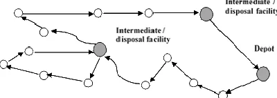
Figure 1: Illustration of A Waste Collection Vehicle Routing Problem
Solid waste is a type of waste that comes from households, streets, constructions, and hygiene debris including recyclable waste such as glass, paper, plastic, and aluminum. Solid waste collection is one of the complex logistic problems endured by municipalities. The operational costs, environmental and health concerns as well as the growing regulation burden have caused municipal and private waste collection companies to improve the collection routes [7] . In developing countries, waste collection is one of the most challenging operational problems [8]. In solid waste collection, as illustrated in Figure 1, wastes are collected from different segmented areas and are transferred to intermediate facilities [3]. A collection vehicle leaves the depot (garage), starts collecting waste from the collection points (customers), and when the vehicle is full, it reaches an intermediate facility for the unloading operation; then it starts with another collection tour and returns to the depot when all collection points are visited or when the constraints of the routing is met. All vehicles must unload waste at intermediate facilities before returning back to the depot without any waste by the end of the day [2]. But there are cases where the unloading process can be done on the next day if the unloading constraint and procedure are applied. In such cases, a vehicle travels from the depot to collect waste from a collection point and continues to the next collection point. It returns to the depot by the end of the day with waste and empties the vehicle at the disposal facility on the next day.
One of the common methods to manage waste collection is by using the vehicle routing problem
(VRP). According to [8], the goal of VRP is to optimize routes without violating any specific constraints such as capacity, time window, number of vehicles, and depots. The routing problem is essential as it deals with cost and time constraints, scheduling as well as satisfying customer demands. Vehicle routing has been an important area of research and was introduced by Dantzig and Ramser in 1959 [9]. Transportation costs denote an average of one to two-thirds of the company’s logistic cost and 15% of the sale price of goods. Thus, solving the vehicle routing problem efficiently is able to save logistic costs [10].
In the case of waste collection, VRP helps to reduce the number of trips and travel distances as well as the reduction of fuel consumption and vehicle emissions [11]. Despite the facts, for the last 40 years, the academic paper researchers about the WCVRP are quite limited [4]. However, today, due to the fast development of new and more efficient optimization and computing methods, they have slowly attracted the attention and interest of academics and practitioners.
Part of their focuses are on two crucial elements in seeking optimum routes. The first is realistic data and constraints such as time, distance, capacity, route, depot, and vehicle fleets [8], as well as the number of trucks, workers, and collection facilities. They are selected from a range of continuous research and analysis.
The second crucial element for route optimization is the formulation of an algorithm. Optimization methods are classified into approximate algorithms and exact algorithms. Optimal or near-optimal solution is generally achieved by using either approximate or exact algorithms. One of the challenges in optimization is VRP is considered as a nondeterministic polynomial time (NP) and hard combinatorial optimization problem.
Since WCVRP is an essential and developing research topic, there are plenty of room for improvement. However, before any advancement can be made, a review is required on problem description and direction of previous researchers in this area.
[image:2.612.101.301.220.291.2]The scope of this review is on solid waste, which are organic and recyclables waste. The waste is classified as residential, commercial and industrial waste. Other types of waste such as hazardous and liquid are not included. This study limits the coverage to the past 11 years of published papers.
The sources for this paper are selected from: (1) academic databases and journals such as Elsevier, Springer, Science Direct, Scopus, and Scientific Research. Keywords used are vehicle routing problem, waste collection, trash collection, rubbish collection, refuse collection, junk collection, garbage collection, methods, algorithms, techniques, heuristic, and metaheuristic.; (2) bibliographies of survey papers and book chapters; (3) books focused on algorithm, waste, and vehicle routing problem. The searching process is confined to articles published from 2005 to 2016 to expose the latest results and trends.
Taking these introductory remarks into account, this paper is organized as follows. Section 2 is devoted to benchmark datasets in waste collection problems. Section 3 deals with waste collection case studies in real-life applications. Classification of constraints on the waste collection problem are discussed in Section 4. Finally, WCVRP methods and algorithms for benchmark datasets and case studies are introduced in Section 5. Section 6 discusses the comparison of research objectives and comparisons of algorithms. As a final point, a conclusion is drawn in Section 7.
2. BENCHMARK DATASETS
[image:3.612.312.525.104.489.2]In reaching the optimum route for the waste collection problem, there are parameters and constraints that need to be identified. However, they are differed with environments such as regions, situations, and climate. Thus, the parameters and constraints collected become the benchmark and are limited for such environment. In particular, this paper discusses the five benchmark datasets used in waste collection. They are the waste collection benchmarks by [12], [13],[14], [15], and [16]
Table 1: Benchmark Datasets
BENCHMARK: [12] , Commercial waste
DETAILS: 22 instances, 48 and 96 customers, and 5 or 7 depot
Ref. Objectives
[2] Maximize route compactness and reduce costs
[17] To improve to multi-depot vehicle routing problem and minimize costs
BENCHMARK: [13], Commercial waste
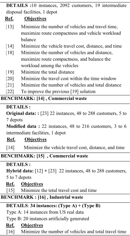
DETAILS :10 instances, 2092 customers, 19 intermediate
disposal facilities, 1 depot
Ref. Objectives
[13] Minimize the number of vehicles and travel time, maximize route compactness and vehicle workload balance
[14] Minimize the vehicle travel cost, distance, and time [18] Minimize the number of vehicles and distance,
maximize route compactness, and balance the workload among the vehicles
[19] Minimize the total distance
[20] Minimize the travel cost within the time window [21] Minimize the number of vehicles and total distance [22] To improve the previous [19] solution
BENCHMARK:[14] , Commercial waste
DETAILS :
Original data: : [23] 22 instances, 48 to 288 customers, 5 to
7 depots
Modified data : 22 instances, 48 to 216 customers, 3 to 6 intermediate facilities, 1 depot
Ref. Objectives
[14] Minimize the vehicle travel cost, distance, and time
BENCHMARK: [15] , Commercial waste
DETAILS :
Hybrid data: [12] + [23] 22 instances, 48 to 288 customers,
5 to 7 depots
Ref.
[15]
Objectives
Minimize the total travel cost and time
BENCHMARK :[16] , Industrial waste
DETAILS: 34 instances: (Type A) + (Type B)
Type A: 14 instances from US real data Type B: 20 instances artificially generated
Ref.
[16]
Objectives
Minimize the number of vehicles and total travel time
As reported in Table 1, there are five established benchmark datasets used in WCVRP. The table provides entrancing information on their waste type, details, and objectives. The benchmark instances introduced by [12] contain 48 and 96 customers and 5 or 7 depots and can be downloaded at http://chairelogistique.hec.ca/en/scientific-data/. [2] and [17] used the instances as the benchmark in their researches.
ISSN: 1992-8645 www.jatit.org E-ISSN: 1817-3195 this benchmark as a waste collection vehicle
routing problem with time window problem. The research objectives were to minimize the number of vehicles and travel time, maximize route compactness, and allocate equal assignment among the vehicles. Researches that refer to [13]’s instances generally have the same objectives, which were to minimize the number of vehicles and travel time, maximize route compactness, and allocate equal assignment among the vehicles. Route compactness is defined as setting all stops into the routes; routes without overlapping is considered more compact as compared to crossover routes.
[18] conducted a research using [13]’s benchmark datasets with the objectives to minimize the total number of vehicles and distance, maximize route compactness, and balance the workload among the vehicles. On the other hand, [14] initially intended to minimize costs such as fixed cost for vehicles, travelling and wage, distance, and time. [19],[20] used the same waste collection problem as in [14]. [21] aimed to reduce the number of vehicles and total distance. [22]’s objective is to improve the previous [19] solution.
This benchmark dataset can be retrieved from: https://sites.google.com/site/logisticslaboratory/rese
arch/research-areas/waste_collection_vrptw_benchmark.
[23] generated 22 instances, 48 to 288 customers, and 5 to 7 depots from those proposed by [12]. Subsequently, [14] modified the set of [23] to suit with the waste collection problem with a single vehicle depot. The new instances comprise 4 to 6 available vehicles, 22 instances of 48 to 216 customers, 3 to 6 intermediate facilities, and a single vehicle depot.
A new benchmark dataset was proposed by [15], which combines instances by [12] and [23]. This is possible because both datasets have the same set of customers. The number of customers and intermediate facilities, the maximum duration, and maximum capacity are taken from [23]’s instances. The number of days of the planning period and service frequencies are taken from [12]’s instances. The main objectives were to minimize the total travel cost and total travel time.
[16] introduced an industrial benchmark dataset with 34 instances; 14 were derived from a real waste collection company in the US and the other 20 were artificially generated. The objectives were
mainly to reduce cost and distance travel as well as to complete tasks within the time window. The benchmark dataset is available at
http://logistics.postech.ac.kr/RR-VRPTW_benchmark.htm.
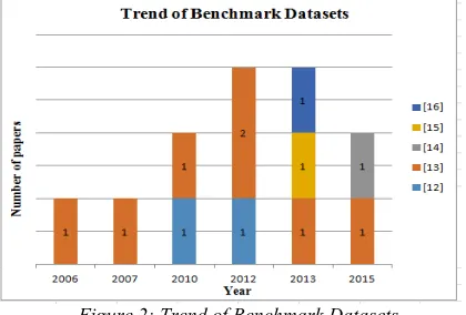
[image:4.612.314.524.201.343.2]Figure 2 shows the trend of studies for benchmark datasets over the years starting from 2006 to 2016.
Figure 2: Trend of Benchmark Datasets
[12] publications are in 2010, and 2012, showing the relevance and interest of researchers that still exist although it was first published 15 years ago. 50% of publications used [13]’s benchmark dataset. The interest of using [13]’s benchmark dataset is increasing as two papers were published in 2012 as compared to one paper in the previous years. Contrary to [12]’s benchmark dataset, the trend showed a horizontal pattern, indicating few interests in using the benchmark dataset. Interestingly, [13]’s benchmark dataset includes the lunch break time window constraint, allowing the data to be complex and reliable to researches. Other benchmark datasets show consistency where [14], [15], and [16] were included in only one publication each.
3. CASE STUDIES
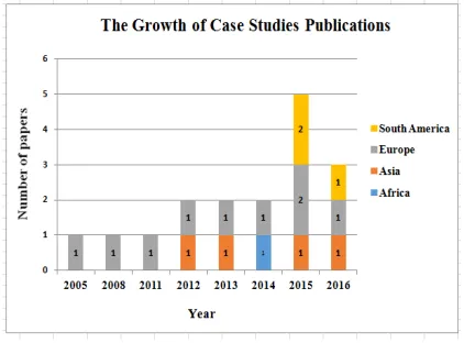
A case study is used to test a solution method and demonstrate the understanding of real-life applications. This paper discusses the municipalities and private companies’ case studies from various countries from four continents. Waste type, details, and results that indicate the performance by each benchmark dataset are tabulated as in Table 2.
expected to increase in the near future. Most of the case studies are mainly from developed countries, but the number of case studies in developing countries is increasing. It is believed to increase due to the environmental awareness, the need for a clean environment and healthy lifestyle, and the availability of modern facilities.
Figure 3: The Growth of Case Study Publications
4. CONSTRAINTS CLASSIFICATION
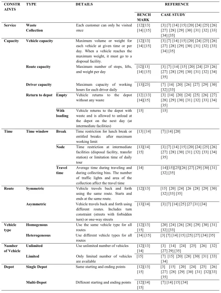
In the previous sections, reviews on the WCVRP benchmark and case studies have been discussed. This section continues with identifying the constraints used in the researches. In general, constraints influence the solution results. The problem becomes more complex and realistic by adding more constraints to the problem. Constraints in waste collection include service, capacity, time, route, vehicle type, number of vehicles, and depot. In most cases, vehicles are not allowed to violate the constraints given.
Service refers to waste collection in which a collection point can only be visited once. Capacity can be categorized as vehicle capacity that holds the maximum volume and weight for each vehicle at any given time [12]. Vehicle volume and weight capacity cannot be violated at any point in the tour [7]. Fuel weights during the consumption distance are also taken into account [36]. When a vehicle is full or has reached the maximum volume, it needs to go to the intermediate facility or landfill to be emptied. Then, it can continue the trip to collect more waste. Vehicle capacity states the maximum number of volume and weight that can be handled per vehicle per day. In route capacity, the maximum number of stops is identified. Vehicles are also allowed to make multiple disposal trips per day [1]. This is to achieve route compactness, where stops are grouped into a route to avoid or
minimize overlapping. Driver capacity is the maximum capacity of working hours for each driver per any given day. This is due to the eight-hour work day limit, permitted by the national legislation [34]. Most vehicles will return to the depot without loading where the last stop is the intermediate facilities. In cases where vehicles return to the depot with loading either fully or partially, they will be emptied the next day. The purpose is to reduce the cost and time constraints. [14] believed that it is seldom optimal for a vehicle to return to its origin depot especially in rural areas.
Time window restricts the time of the vehicles leaving the depot, in which the vehicles should only leave the depot after the start time and they must return to the depot within the finish time. It is also considered that all vehicles leave the depot at the same time without a queuing problem. Lunch break is considered as the time window where drivers are given a specific time to have lunch at the nearby area. Traffic congestion is considered as one of the dynamic constraints since it affects vehicle travel time. The area of collection in urban areas usually takes more travel time compared to rural areas. Time windows are divided into two types, which are hard time and soft time windows. Normally, in hard time window, vehicles must wait until the start of the time window before service can commence [37]. In contrast, soft time window allows vehicles to violate the time window constraint, but at the price of some penalty [38].
ISSN: 1992-8645 www.jatit.org E-ISSN: 1817-3195 applications, asymmetric routes need to be
considered because of the one-way streets.
Subject to the different waste characteristics and complexity of the problem, different types of vehicles are used for waste collection [3]. The vehicle type can be categorized as homogeneous and heterogeneous. The number of vehicles can be categorized as unlimited and limited. The constraints with unlimited vehicles allow waste collection without limiting the number of vehicles. However, limited constraints require the waste to be collected using a specific number of vehicles provided. Initially, vehicles are stationed at the depot, and for a single depot, a vehicle starts from a depot and must return to the same depot at the end of the day [14]. On the other hand, a multi-depot allows vehicles to start and end at different locations. In a multi-depot situation, it is usually a mix of urban and rural regions, and therefore, it is not always optimal for a vehicle to return to the same depot [7].
Table 3 summarizes the main constraints used in the benchmark and case study datasets reviewed in the previous sections. As shown in the table, most constraints are used extensively, but several of the constraints need to be considered such as driver capacity, return to depot with loading, lunch break, travel time, and asymmetric route. Several situations allow vehicles to return to the depot with loading and can be emptied on the next day. Subsequently, it reduces travel distance and cost, especially for urban WCVRP.
5. METHODS AND ALGORITHMS
This section analyzes different methods and algorithms used to solve the previous waste collection benchmark datasets and case studies. Methods and WCVRP are associate with each other in order to find the minimum distance and reducing cost. Main objective of WCVRP is to optimize the routes and decrease the total cost of the routes by reducing travel period with minimum distance along with capacity constraints and vehicle used. The shortest distance travelled by all the vehicles without violating any rules is considered as feasible solution [39].
5.1 Benchmark Datasets Methods and Results
Table 4 outlines the benchmark datasets, methods, and results used by researchers with engaging results. Researchers used benchmark datasets to achieve their objectives and most of the
researchers produced interesting results by using different methods and algorithms. The previous studies are grouped according to the benchmark datasets, and comparisons on the algorithms used and results against each study are presented. Interestingly, most of the results show improvement and some of them outperformed the best known solutions.
5.2 Case Studies Methods and Results
Pertinent to the previous section above, this section reveals the results of solutions from real-life waste collection problems using various methods and algorithms. Table 5 below presents the results from classification of case studies by continents along with the methods and algorithms used.
Table 5 summarizes the methods and algorithms used in case studies according to continent and countries. The results reveal the success of each case study. Importantly, billions of dollars have been saved and total operational costs have been reduced. A few researchers measured the reduction of carbon dioxide emissions, and thus indicated the successfulness in taking a step forward in integrating environmental awareness as one of the research objectives.
6. DISCUSSION
In this section, the research objectives and methods used in previous researches are discussed.
6.1 Comparison of Research Objectives
The objectives in vehicle routing problems are categorized as economical, climate and environmental (ecosystem and health). The most common objective in waste collection is economical with the purpose of minimizing the cost, time, travel distance, routes or number of vehicles.
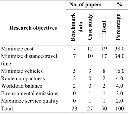
The results in Table 6 shows that more than two third of the researchers concentrated on how to minimize costs, minimize distance or travel time, and minimize vehicle numbers, but less than one third have taken into consideration to maximize route compactness, workload balance, environmental emissions, and service quality. Route compactness is how stops are grouped together to form a route. Routes without crossovers are more compact as compared to routes with crossovers. Routes that have many crossovers are considered less compact compared to those without overlapping. Some researchers mentioned route compactness implicitly and it has not become the vital or important element in their research; whereas a few researchers expressed explicitly its details in their studies and it has become a part of their contribution
Table 6: Statistics on Research Objectives
The environmental issues, quality of service, and maximizing the collection of waste were mentioned by a few researchers, but were barely stressed explicitly by some of the researchers. Respectively, the combination of optimal solutions from the quantity of waste collected, number of vehicles, and vehicle travel distance ultimately reduce the environmental emissions. The quality of service is indicated by frequency and balanced period of each visit at each collection point. To correspond, the environmental issue, quality of service and workload balance among the vehicles are rare, but are considered to be significant issues.
Relevant to Table 6, some researchers focused on mono-objective, whereas modern waste collection today sets its purpose to be multi-objective. In multi-objective optimization problems, two or more
goals or parameters have the ability to affect the overall result. But frequently, each of these objectives might affect each other in a complicated nonlinear way.
Hence, this is the gap and challenge for researchers to find a set of values that is able to produce optimized results. Multi-objective serves as a significant contribution to waste management not only for economical purpose, but the effects to environmental issues such as emissions and noise. For that reason, there is a need for researchers to incorporate these objectives together.
6.2 Comparison of Methods
The previous sub-topics have analyzed two main relationships, which are the benchmark datasets and the solution methods. The relationships are concluded by analyzing the relationships from different point of views, which are the data and their relation to algorithms.
Algorithms are categorized into approximate and exact algorithms. Approximate algorithm is preferable and commonly used in practice as it is able to find very near-optimal solutions for large-scale problems within a very satisfactory computational time. Since 1980s, there are a variety of approximate algorithms, which include heuristics and metaheuristics that efficiently solve different variants of VRP. Heuristic is a classic VRP. Some of the common types of metaheuristics are Simulated Annealing, Tabu Search, Variable Neighborhood Search, Large Neighborhood Search, Evolutionary Algorithms, and Ant Colonies [40], [41]. Heuristics and metaheuristics have less computational time for solving problems as compared to exact methods. Heuristics are specific algorithms for a problem; to find good solutions, not necessarily the optimal one. A heuristic method is capable to handle a very large and complex problem with effective computational time. Whereas metaheuristics have the capacity of avoiding local optimums as they have better exploration in solution space. Exact algorithms can only tackle problems usually of a small scale [38] and some of the commonly used algorithms in VRP are and-bound, and-cut, and branch-and-price algorithms [40].
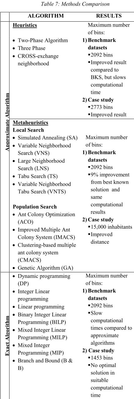
Table 7 compares between approximate and exact algorithms used based on the above benchmark datasets and case studies. The number of customers to be served is relative to the selection of algorithms and results. It also presents the No. of papers %
Research objectives
B
en
ch
m
a
rk
d
a
ta
C
a
se
s
tu
d
y
T
o
ta
l
P
er
ce
n
ta
g
e
Minimize cost
Minimize distance/travel time
Minimize vehicles
7 7
5 12 10
3 19 17
8 38.0 34.0
16.0 Route compactness 2 0 2 4.0 Workload balance
Environmental emissions 2 0
0 1
2 1
4.0 2.0 Maximize service quality 0 1 1 2.0
ISSN: 1992-8645 www.jatit.org E-ISSN: 1817-3195 comparisons of algorithms used in previous benchmark datasets and case studies. Significantly, it shows the relation between the algorithms and the total numbers of bins.
In order to compare the relevance of instance size and the algorithms, this research selects the maximum number of collections or bins. The benchmark dataset introduced by [13] consists of 2092 bins and has been tested by researchers using approximate and exact methods. From the analyses, basically, it was proven that heuristics and metaheuristics are capable to produce better results as compared to exact methods for big-scale instances with respect to the constraints used. The results also show that by using approximate algorithms in the benchmark dataset, the computational time is faster than when using exact algorithms. In contrast, there is no optimal solution in a suitable computational time for exact algorithms. When it comes to large-scale instances, approximate algorithms have the capability to cater the data and produce a quality result as compared to exact algorithms. Therefore, the strength of the metaheuristic algorithms is the capability in optimizing large-scale data with better computational time.
7. CONCLUSION
With respect to this research aim, this study has identified several contributions. Firstly, some of the constraints that should be considered are highlighted. Secondly, this investigation concluded that most papers have mono objectives mainly on minimizing cost or distance travelled. The environmental issue and quality of service are rare but are considered as significant issues. Additional objective of reducing environmental emissions or maximizing service quality can be incorporate and becomes multi objectives research in WCVRP field. Multi objectives studies can serve as a significant contribution for both the economic and environmental issues.
[image:8.612.84.299.92.728.2]Thirdly, results showed the relationship of methods with the size of instance. The size of benchmark data or case study is one of the factors that affect the performance by using exact methods or approximate methods. Exact methods are suitable for small dataset size whereas heuristic and metaheuristic methods cater for bigger size of data. The strength of the approximate methods is the capability in providing good result for large-scale data.
Table 7: Methods Comparison
ALGORITHM RESULTS
A p p ro x im a te A lg o ri th m
Heuristics Maximum number
of bins: • Two-Phase Algorithm
• Three Phase • CROSS-exchange neighborhood 1)Benchmark datasets 2092 bins Improved result compared to BKS, but slows computational time
2)Case study 2773 bins Improved result Metaheuristics
Local Search
• Simulated Annealing (SA) • Variable Neighborhood
Search (VNS) • Large Neighborhood
Search (LNS) • Tabu Search (TS) • Variable Neighborhood
Tabu Search (VNTS)
Population Search • Ant Colony Optimization
(ACO)
• Improved Multiple Ant Colony System (IMACS) • Clustering-based multiple
ant colony system (CMACS)
• Genetic Algorithm (GA)
Maximum number of bins: 1)Benchmark datasets 2092 bins 9% improvement from best known solution and same computational results 2)Case study
15,000 inhabitants Improved distance E x a ct A lg o ri th m
• Dynamic programming (DP)
• Integer Linear programming • Linear programming • Binary Integer Linear
Programming (BILP) • Mixed Integer Linear Programming (MILP) • Mixed Integer
Programming (MIP) • Branch and Bound (B &
B) Maximum number of bins: 1)Benchmark datasets 2092 bins Slow computational times compared to approximate algorithms 2) Case study
Subsequently, there is an increasing pattern of trends using benchmark data and case studies in WCVRP. Most of publications used benchmark data that include the real environment constraints of time window and lunch break. More case studies came from developing countries indicating the interest for a healthy lifestyle and environmental awareness.
The result of this study potentially represents a step forward and guidance for researchers in WCVRP.
ACKNOWLEDGMENT
The authors wish to thank the Ministry of Higher Education Malaysia for funding this study under the Fundamental Research Grant Scheme, S/O code 13240 and RIMC, Universiti Utara Malaysia, Kedah, for the administration of this study.
REFERENCES
[1] M. Faccio, A. Persona, and G. Zanin, “Waste collection multi objective model with real time traceability data,” Waste Manag., vol. 31, no. 12, pp. 2391–2405, 2011.
[2] J. Liu and Y. He, “A clustering-based multiple ant colony system for the waste collection vehicle routing problems,” Proc. - 2012 5th Int. Symp. Comput. Intell. Des. Isc. 2012, vol. 2, pp. 182–185, 2012.
[3] S. Das and B. K. Bhattacharyya, “Optimization of municipal solid waste collection and transportation routes,” Waste Manag., vol. 43, pp. 9–18, 2015.
[4] H. Han, E. Ponce-cueto, and E. Management, “Waste Collection Vehicle Routing Problem : Literature Review,” Promet - Traffic Transp., vol. 27, no. 4, pp. 345–358, 2015.
[5] S. Fooladi, H. Fazlollahtabar, and I. Mahdavi, “Waste Collection Vehicle Routing Problem Considering Similarity Pattern of Trashcan,” Int. J. Appl. Oper. Res., vol. 3, no. 3, pp. 105– 111, 2013.
[6] J. Beliën, L. De Boeck, and J. Van Ackere, “Municipal Solid Waste Collection and Management Problems: A Literature Review,” Transp. Sci., vol. 48, no. 1, pp. 78–102, 2014. [7] I. Markov, S. Varone, and M. Bierlaire,
“Vehicle Routing for a Complex Waste Collection Problem,” 14th Swiss Transp. Res. Conf., no. April, pp. 1–25, 2014.
[8] J. Caceres-Cruz, P. Arias, D. Guimarans, D. Riera, and A. A. Juan, “Rich Vehicle Routing Problem,” ACM Comput. Surv., vol. 47, no. 2, pp. 1–28, 2014.
[9] Ç. Koç, T. Bektaş, O. Jabali, and G. Laporte, “Thirty years of heterogeneous vehicle routing,” Eur. J. Oper. Res., vol. 249, no. 1, pp. 1–21, 2016.
[10] N. Labadie and C. Prins, “Vehicle Routing Nowadays : Compact Review and Emerging Problems,” in Production Systems and Supply Chain Mangement in emerging Countries : Best Practices, Springer-Verlag Berlin Heidelberg, 2012, pp. 141–166.
[11] J. R. Kinobe, T. Bosona, G. Gebresenbet, C. B. Niwagaba, and B. Vinner, “Optimization of waste collection and disposal in Kampala city,” Habitat Int., vol. 49, pp. 126–137, 2015. [12] J. F. Cordeau, M. Gendreau, and G. Laporte, “A
tabu search heuristic for periodic and multi-depot vehicle routing problems,” Networks, vol. 30, pp. 105–119, 1997.
[13] B.-I. Kim, S. Kim, and S. Sahoo, “Waste collection vehicle routing problem with time windows,” Comput. Oper. Res., vol. 33, no. 12, pp. 3624–3642, 2006.
[14] I. Markov, S. Varone, and M. Bierlaire, “The waste collection VRP with intermediate facilities , a heterogeneous fixed flee and a fexible assignment of origin and destination depot,” Rep. TRANSP-OR, 2015.
[15] V. Hemmelmayr, K. F. Doerner, R. F. Hartl, and S. Rath, “A heuristic solution method for node routing based solid waste collection problems,” J. Heuristics, pp. 1–28, 2013. [16] J. Wy, B. Kim, and S. Kim, “The rollon –
rolloff waste collection vehicle routing problem with time windows,” Eur. J. Oper. Res., vol. 224, no. 3, pp. 466–476, 2013.
[17] J. Liu, D. Liu, M. Liu, and Y. He, “An improved multiple ant colony system for the collection vehicle routing problems with intermediate facilities,” Proc. World Congr. Intell. Control Autom., pp. 3078–3083, 2010. [18] B. Ombuki-Berman, “Waste collection vehicle
routing problem with time windows using multi-objective genetic algorithms,” Proc. Third, no. APRIL, 2007.
ISSN: 1992-8645 www.jatit.org E-ISSN: 1817-3195 Comput. Oper. Res., vol. 37, no. 12, pp. 2270–
2280, 2010.
[20] K. Buhrkal, A. Larsen, and S. Ropke, “The waste collection vehicle routing problem with time windows in a city logistics context,” Procedia - Soc. Behav. Sci., vol. 39, pp. 241– 254, 2012.
[21] R. Islam and M. S. Rahman, “An ant colony optimization algorithm for waste collection vehicle routing with time windows, driver rest period and multiple disposal facilities,” 2012 Int. Conf. Informatics, Electron. Vision, ICIEV 2012, pp. 774–779, 2012.
[22] A. M. Benjamin and J. E. Beasley, Metaheuristics with disposal facility positioning for the waste collection VRP with time windows, vol. 7, no. 7. Springer, 2013.
[23] B. Crevier, J. F. Cordeau, and G. Laporte, “The multi-depot vehicle routing problem with inter-depot routes,” Eur. J. Oper. Res., vol. 176, no. 2, pp. 756–773, 2007.
[24] D. Otoo, S. K. Amponsah, and C. Sebil, “Capacitated clustering and collection of solid waste in kwadaso estate, Kumasi,” J. Asian Sci. Res. J., vol. 4(8), no. 8, pp. 460–472, 2014. [25] J. Liu and Y. He, “Ant colony algorithm for
waste collection vehicle arc routing problem with turn constraints,” Intell. Secur. (CIS), 2012 Eighth, 2012.
[26] Y. L. Hou Ming Hou, Jia Shu Li, Xiao Nan Zhang, “The Study on Hybrid Scheduling Optimization of Industrial Solid Waste Recycling Vehicle Routing with Time Window.pdf,” Inf. Technol. Journal, 2013. [27] L. H. Son and A. Louati, “Modeling municipal
solid waste collection: A generalized vehicle routing model with multiple transfer stations, gather sites and inhomogeneous vehicles in time windows,” Waste Manag., 2016.
[28] N. V. Karadimas, G. Kouzas, I. Anagnostopoulos, and V. Loumos, “Urban solid waste collection and routing: The ant colony strategic approach,” Int. J. Simul. Syst. Sci. Technol., vol. 6, no. 12–13, pp. 45–53, 2005. [29] M. P. Fanti, A. M. Mangini, L. Abbatecola, and
W. Ukovich, “Decision Support for a Waste Collection Service with Time and Shift Constraints,” Am. Control Conf., pp. 2599– 2604, 2016.
[30] T. Bianchi-Aguiar, M. A. Carravilla, and J. F. Oliveira, “Vehicle Routing for Mixed Solid Waste Collection,” VII ALIO–EURO – Work. Appl. Comb. Optim., pp. 137–140, 2011.
[31] J. Bautista, E. Fernandez, and J. Pereira, “Solving an urban waste collection problem using ants heuristics,” Comput. Oper. Res., vol. 35, no. 9, pp. 3020–3033, 2008.
[32] J. R. Gomez, J. Pacheco, and H. Gonzalo-Orden, “A Tabu Search Method for a Bi-Objective Urban Waste Collection Problem,” Comput. Civ. Infrastruct. Eng., vol. 30, no. 1, pp. 36–53, 2015.
[33] P. C. Yesica Xiomara, Daza Cruz, Johana Andrea and E. R. Santana, “A mixed integer optimization model to design a selective collection routing problem for domestic solid waste,” IEEE, 2015.
[34] T. P. B. Vecchi, D. F. Surco, A. A. Constantino, M. T. A. Steiner, L. M. M. Jorge, M. A. S. S. Ravagnani, and P. R. Paraíso, “A sequential approach for the optimization of truck routes for solid waste collection,” Process Saf. Environ. Prot., vol. 102, pp. 238–250, 2016.
[35] P. A. Miranda, C. A. Blazquez, R. Vergara, and S. Weitzler, “A novel methodology for designing a household waste collection system for insular zones,” Transp. Res. Part E Logist. Transp. Rev., vol. 77, pp. 227–247, 2015. [36] T. V. Anagnostopoulos and A. Zaslavsky,
“Effective waste collection with shortest path semi-static and dynamic routing,” Lect. Notes Comput. Sci. (including Subser. Lect. Notes Artif. Intell. Lect. Notes Bioinformatics), vol. 8638 LNCS, pp. 95–105, 2014.
[37] A. Sbihi and R. W. Eglese, “The Relationship between Vehicle Routing & Scheduling and Green Logistics - A Literature Survey,” Lancaster Univ. Manag. Sch., pp. 1–24, 2007. [38] C. Lin, K. L. Choy, G. T. S. Ho, S. H. Chung,
and H. Y. Lam, “Survey of Green Vehicle Routing Problem: Past and future trends,” Expert Syst. Appl., vol. 41, no. 4 PART 1, pp. 1118–1138, 2014.
[39]R. Yesodha and T. Amudha, “A Study on Bio-Inspired Metaheuristics for Solving Vehicle Routing Problem,” Indian J. Sci. Technol., vol. 8, no. October, pp. 1–9, 2015.
[40] S. N. Kumar, “A Survey on the Vehicle Routing Problem and Its Variants,” Intell. Inf. Manag., vol. 04, no. 03, pp. 66–74, 2012.
Table 2: Case Studies Grouped by Continents
COUNTRY DETAILS REF. OBJECTIVES
AFRICA
Ghana • Residential waste, 590,240 liters waste bins, 4.2 tons of solid waste per day, 18,000 citizens
[24] Minimize the total cost and distance
ASIA
China • Commercial waste, Vehicle load capacity (2t, 5t, 8t),584 vertices
• 371 edges, 473 arcs, 95 required links (19855 m), 80,000 citizens
[25] Minimize the travel distance
China • Industrial waste , Number of vehicles: 349, Total costs (travelling, handling, time penalty) are 861,370.6
[26] Minimize the costs for vehicles, travel, handling, and penalty
India • Residential waste, 65 collection centers, 50 transfer stations, 100 points, Total distance: 126.15 km, Vehicle capacity: 4-5 tons
[3] Minimize collection and transportation costs
Vietnam • Residential waste, Tricycle capacity: 6601 bins (170kg) or 2401 bins (140kg/bin), Forklift and hook-lift capacity: 9 tons
[27] Maximize the quantity of waste collected and minimize the environmental emissions (reduce the number of vehicles and travel distance)
EUROPE
Austria • Residential waste, 3 instances, First instance (387 customers, 2 vehicles, 3 IF), Second instance (184 customers, 1 vehicle, 1 IF), Third instance (78 customers, 1 vehicle, 2 IF)
[15] Minimize the total travel cost and time
Denmark • Commercial waste, 8 vehicles, 3 disposals, 228 customers, Drivers working hours less than 9 hours
[20] Minimize the travel cost within the time window
French • Residential waste, 15 instances, 150 containers [7] Minimize the costs, distance, and time Greece • Commercial waste, 100 loading spots, 0.5 km2, 8500
citizens, 3800 tons solid waste per year
[28] Minimize the cost and number of vehicles
Italy • Residential waste, 2773 bins, 1491 pick-up positions, Vehicle capacity: 102 bins, Working time: 6 hours, Each node less than 200 minutes
[29] Minimize the distance
Portugal • Residential waste, 5 vehicles, 994 containers, 6 working days per week
[30] Minimize the operation cost and distance travel
Spain • Residential waste, 5 trucks, Capacity: 25 cubic meters per vehicle, Road length is 55,993m with 220 edges and 459 arcs
[31] Minimize the travel distance and total cost
Spain • Residential waste, 4 real instances, 48 villages [32] Minimize the transportation costs and maximize service quality
Switzerland • Commercial waste, 15 instances, 35 tours, 7 to 38 containers, 4 dumps per tour
[14] Minimize the vehicle cost and travel distance
SOUTH AMERICA
Colombia • Residential waste, 13 blocks, 51 corners, 1453 houses, 3860 users, 2 trucks (23 km/h, 2800 kg), 1 wheelbarrow (4.4 km/h, 120 kg).
[33] Maximize the amount of waste collected by taking into consideration the city’s real situation
Brazil • Residential waste, 2 vehicles, 90,000 citizens, Vehicle capacity: 17 tons, 6 tons, Collection area: 71,420m
[34] Minimize the travel distance and total cost
Chile • Residential waste, 20 islands, 33 sites, 300 to 1200 inhabitants per island
ISSN: 1992-8645 www.jatit.org E-ISSN: 1817-3195 Table 3: Constraints in Waste Collection Vehicle Routing Problem
CONSTR AINTS
TYPE DETAILS REFERENCE
BENCH MARK
CASE STUDY
Service Waste
Collection
Each customer can only be visited once
[12][13] [14] [15]
[3] [7] [14] [15] [20] [24] [25] [26] [27] [28] [29] [30] [31] [32] [33] [34] [35]
Capacity Vehicle capacity Maximum volume or weight for
each vehicle at given time or per day. When a vehicle reaches the maximum weight, it must go to a disposal facility.
[12][13] [14] [15]
[3] [7] [14] [15] [20] [24] [25] [26] [27] [28] [29] [30] [31] [32] [33] [34] [35]
Route capacity Maximum number of stops, lifts,
and weight per day
[12][13] [14] [15]
[3] [7] [14] [15] [20] [24] [25 [26] [27] [28] [29] [30] [31] [32] [34] [35]
Driver capacity Maximum capacity of working
hours for each driver daily
[13][23] [7] [14] [20] [26] [27] [29] [30] [32] [33]
Return to depot Empty Vehicle returns to the depot
without any waste
[12] [13] [14][15]
[3] [14] [20] [24] [25] [26] [27] [28] [29] [30] [31] [32] [33] [34] [35]
With loading
Vehicle returns to the depot with waste and is allowed to unload at the depot on the next day (at intermediate facilities)
[15] [15]
Time Time window Break Time restriction for lunch break or
entitled breaks after maximum working limit
[13] [14] [7] [14] [20]
Node Time restriction at intermediate
facilities (disposal facility, transfer station) or limitation time of daily tour
[13][14] [15]
[3] [7] [14] [15] [20] [24] [25] [26] [27] [28] [30] [31] [32] [33] [34] [35]
Travel time
Average time during traveling and during collecting bins. The number of traffic lights and area of the collection affect the travel time
[14] [14][15][25][26] [27] [29] [30] [31] [32] [35]
Route Symmetric Vehicle travels back and forth
using the same route. Starts and ends at the same route.
[12][13] [15] [20] [24] [26 [28] [29] [30] [32] [33] [35]
Asymmetric Vehicle travels back and forth using
different routes. Includes turn constraint (streets with forbidden turn) or one-way streets
[13][14] [3] [7] [14] [25] [27 [31] [34]
Vehicle type
Homogenous Use the same vehicle type for all
routes
[12][13] [15]
[20] [24] [26] [28] [29] [30] [31] [32] [33]
Heterogeneous Use different vehicle types for all
routes
[14] [15] [3] [7] [14] [15] [25] [27] [34] [35]
Number of Vehicle
Unlimited Use unlimited number of vehicles [12][13]
[14]
[3] [14] [24] [25] [26] [32] [27] 29] [35]
Limited Only limited number of vehicles
are available
[15] [7] [15] [20] [28] [30] [31] [33] [34]
Depot Single Depot Same starting and ending points [12][13]
[15]
[3] [15] [20] [24] [25] [26] [27] [28] [29] [30] [31] [32][33] [35]
Multi-Depot Different starting and ending points [12][14]
[15]
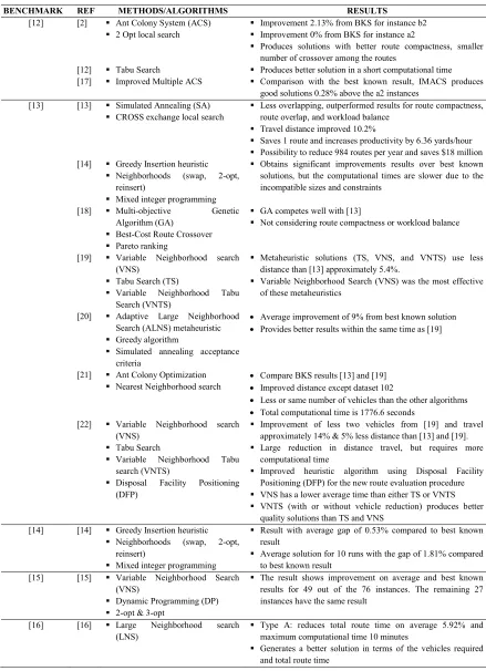
Table 4: Benchmark Datasets, Methods and Results
BENCHMARK REF METHODS/ALGORITHMS RESULTS
[12] [2] Ant Colony System (ACS)
2 Opt local search
Improvement 2.13% from BKS for instance b2 Improvement 0% from BKS for instance a2
Produces solutions with better route compactness, smaller number of crossover among the routes
[12] Tabu Search Produces better solution in a short computational time [17] Improved Multiple ACS
Comparison with the best known result, IMACS produces good solutions 0.28% above the a2 instances
[13] [13] Simulated Annealing (SA) CROSS exchange local search
Less overlapping, outperformed results for route compactness, route overlap, and workload balance
Travel distance improved 10.2%
Saves 1 route and increases productivity by 6.36 yards/hour Possibility to reduce 984 routes per year and saves $18 million [14] Greedy Insertion heuristic
Neighborhoods (swap, 2-opt, reinsert)
Mixed integer programming
Obtains significant improvements results over best known solutions, but the computational times are slower due to the incompatible sizes and constraints
[18] Multi-objective Genetic Algorithm (GA)
Best-Cost Route Crossover Pareto ranking
GA competes well with [13]
Not considering route compactness or workload balance
[19] Variable Neighborhood search (VNS)
Tabu Search (TS)
Variable Neighborhood Tabu Search (VNTS)
Metaheuristic solutions (TS, VNS, and VNTS) use less distance than [13] approximately 5.4%.
Variable Neighborhood Search (VNS) was the most effective of these metaheuristics
[20] Adaptive Large Neighborhood Search (ALNS) metaheuristic Greedy algorithm
Simulated annealing acceptance criteria
• Average improvement of 9% from best known solution
• Provides better results within the same time as [19]
[21] Ant Colony Optimization Nearest Neighborhood search
• Compare BKS results [13] and [19]
• Improved distance except dataset 102
• Less or same number of vehicles than the other algorithms
• Total computational time is 1776.6 seconds [22] Variable Neighborhood search
(VNS) Tabu Search
Variable Neighborhood Tabu search (VNTS)
Disposal Facility Positioning (DFP)
Improvement of less two vehicles from [19] and travel approximately 14% & 5% less distance than [13] and [19]. Large reduction in distance travel, but requires more computational time
Improved heuristic algorithm using Disposal Facility Positioning (DFP) for the new route evaluation procedure VNS has a lower average time than either TS or VNTS VNTS (with or without vehicle reduction) produces better quality solutions than TS and VNS
[14] [14] Greedy Insertion heuristic Neighborhoods (swap, 2-opt, reinsert)
Mixed integer programming
Result with average gap of 0.53% compared to best known result
Average solution for 10 runs with the gap of 1.81% compared to best known result
[15] [15] Variable Neighborhood Search (VNS)
Dynamic Programming (DP) 2-opt & 3-opt
The result shows improvement on average and best known results for 49 out of the 76 instances. The remaining 27 instances have the same result
[16] [16] Large Neighborhood search (LNS)
Type A: reduces total route time on average 5.92% and maximum computational time 10 minutes
ISSN: 1992-8645 www.jatit.org E-ISSN: 1817-3195 Table 5: Case Studies, Methods and Results
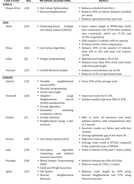
CASE STUDY REF. METHODS/ALGORITHMS RESULT
AFRICA
Ghana Africa [24] Ant Colony Optimization Nearest Neighborhood
Reduces vehicles from 8 to 6
Reduces 40% of vehicle distance travelled per week
Reduces operational time and costs ASIA
China [25] Clustering-based multiple
ant colony system (CMACS)
Saves routes length at 89984.96m (with turn constraint) and 92330.04m (without turn constraint), which are 31.1% and 31.9%, respectively
Only requires 3 vehicles with 6t capacity Produces better route compactness
China [26] Ant Colony Algorithm Reduces 24% of the number of vehicles
from 349 to 265 and total cost reduces 22.6%
India [3] Integer programming Optimal road length is 58.33 km
Reduces more than 30% of the total waste collection path length
Vietnam [27] ArcGIS Network Analyst Reduces travel distance by 16.4%
Reduces 14.3% of operational time EUROPE
Austria [15] Variable neighborhood
search (VNS)
Dynamic programming Clarke and wright
Saves 25% of the average costs
Denmark [20] Adaptive Large
Neighborhood Search
(ALNS) metaheuristic Greedy algorithm
Simulated annealing
acceptance criteria
Improves routes by 8-13%
Solution quality improves 30% to 45%
French [7] Greedy insertion
Neighborhood (swap, 2-opt, reinsert)
Able to solve all instances and reach optimal solution with computational time of 1 second
Heuristic results are better and with less runtime
Average optimality gap of less than 2%
Greece [28] Ant Colony System (ACS) Improves routes by 24%
Average route result is 8725m compared to the empirical route of 9850m
Italy [29] Two-phase algorithm
(clustering and farthest insertion heuristic)
Saves 3 vehicles (15%) and 7 routes (18%)
Portugal [30] Mixed Integer Programming
(MIP)
Clark and Wright heuristics
Reduces distance by 26% (610 km) Reduces route by 3.8% ( 1 route)
Spain [31] Ant System
Nearest Neighborhood
Heuristic
Nearest insertion heuristic Computational time for Nearest Neighborhood is much smaller than Nearest insertion
Reduces route length to 17,000 km per year
Spain [32] Tabu Search (TS)
Sweep algorithm
Reduces the total transport cost by 34% Maximizes the service quality by 36% Switzerland [14] Greedy Insertion heuristic
Neighborhoods (swap, 2-opt, reinsert)
Mixed integer programming (MIP)
Ranges of computational times are from 0.05 to 7.58 s. and an average of 1.21 s. Per instance improvement of average from 1.73% to 34.91% and mean of 14.64% Estimation on financial savings are from 300,000 USD annually for labor and fuel costs
SOUTH AMERICA
Colombia [33] Mixed integer programming
(MIP)
Total waste collected is 604.43 kg and 6891.19 meters
No optimal solution in a reasonable computational time
Brazil [34] Mixed Integer Linear
Programming (MILP) Binary Integer Linear Programming
Reduces 1.5% in total distance for undifferentiated collection. Saves US $3825 per year
Reduces 7.5% in total distance for selective collection. Saves US $4146 per year
Reduces carbon dioxide emissions of approximately 914 kg per year
Chile [35] Mixed Integer Programming
(MIP)
Branch and Bound (B&B)