WSN BASED SENSING MODEL FOR SMART CROWD MOVEMENT WITH IDENTIFICATION: AN EXTENDED STUDY

SLIDING MODE OBSERVER FOR A CLASS OF

BIOCHEMICAL PROCESS

1

AMEL BARHOUMI, 1TAOUFIK LADHARI, 1SALIM HADJ SAID AND 1FAOUZI M’SAHLI

1

ESIER, Ibn Eljazar, ENIM, Monastir 5000, Tunisia E-mail: [email protected]

ABSTRACT

In this paper, a design of Sliding Mode Observer (SMO) of a class of biochemical processes is proposed. Indeed, nonlinear observers for the estimation of the substances are presented and the estimation of non-measured states in waste water treatment process is addressed. The proposed observers are very successful in accurately estimating states variables. Specifically, sliding mode observer has been investigated for this class of nonlinear systems. Moreover, they are very easy to implement and to calibrate in order to estimate non measurable state. The sliding mode observer is compared with High Gain Observer (HGO) and Extended Kalman Filter (EKF). The performance of the sliding mode observer is illustrated through numerical simulations. The simulation results for the bioreactor application demonstrate the effectiveness of the proposed observer.

Keywords: Sliding mode observer, biochemical process, nonlinear systems, wastewater treatment, High gain, EKF.

1. INTRODUCTION

In the field of biochemical research, there has been a growing interest on biotechnological

processes. These processes require high

performance control techniques due to increased demands on productivity, product quality and environmental responsibility. Most of the chemical processes are inherently nonlinear and a variety of nonlinear control design strategy has been proposed. However, the application of computer control algorithms for biotechnological process suffers from the difficulty of modeling the growth kinetics of microorganisms and the lack of reliable, sterilizable and robust sensors for the online measurements of process key variables such as biomass, substrate and product concentrations [1,2].

The non-measurable variables in a bioreactor are obtained using indirect techniques [1]. Some of these approaches involved batchwise analyses which are done manually. Therefore, these techniques are time consuming, require a lot of manpower and many results in very expensive solutions as far as the measurements of very specific compounds are concerned [1,3].

One way to avoid these problems is to use estimation strategies. The state estimation of nonlinear systems has been an active field of

research in the last few decades. The works in [1,2,3,4,5,6,7] presented some fundamental results on state estimation of systems via state transformation and nonlinear observer.

In [2], a high-gain observer has been proposed for a general class of single output systems that is

uniformly observable. The approach was

generalized to a more general class of nonlinear systems in [3] and [4]. Indeed, in [4], a constant gain observer is proposed for a special class of nonlinear systems that does not require the nonlinear transformation.

Many of these strategies, which are interested to estimate non-measurable states and disturbances for partially known systems, are based on the Extended Kalman Filter (EKF) and variations theorem [18, 22]. The EKF is an extension of the linear Kalman filter to the case where the system is described in the state space by a nonlinear differential equation. Its design is based on a local linearization system around a reference trajectory [18].

Variants like EKF constant gain were designed to avoid long calculations related to updating the state estimates and covariance matrices.

the variableψ . But, we have difficulty of obtaining a triangular structure even in the case where such a structure is theoretically accessible by a coordinate transformation. And, sensibility in the noise of measure if the gain is chosen too large.

In the modern industry, the development of new techniques to get online estimates of the uncertainty terms in chemical reactors has been advanced. Indeed, as presented in [5, 6] a Sliding Mode Observers (SMO) are designed for a class of nonlinear uncertain continuous and discrete-time systems.

Intense progress was made in the field of observers of nonlinear system [5, 6, 12, 13]. More preferably, Farza and al,[10,11] had successfully developed a simple nonlinear observer for online estimation of the reaction rates in chemical or biochemical reactors.

These techniques use filtering and calorimetric balances. The advantage of these approaches is their easy computational implementation. In the spirit of calorimetric balances, another kind of observer structures can be used is the sliding mode observers.

SMO are robust observers which estimate the state of nonlinear systems. They are well suited for these systems. The main advantages of SMO, over a linear observer such as Luenberger observer, is that SMO can be made considerably more robust to parametric uncertainty, external disturbances and noisy measurements [8].

In this paper, a sliding mode observer is proposed for a biotechnological system. This work is based on [13]. Indeed, this observer is used to estimate the xenobiotic substratum in a biochemical reaction. The main contribution is the design of this observer and comparing it to others in order to show his excellent global properties. To ensure a suitable basis for comparison, different cases are designed (with and without perturbation, adding noise measurement…) and verified with the same test imposed by the biochemical reaction in the system. This observer aroused a lot of interest thanks to his adaptation to a real time use and its capacity to realize good performances.

This work is organized as follows. In the next section, the class of bioprocesses to be studied is discussed and a precise statement of the problem is presented. Section III presents the mathematical model. Then, in section IV we give the design of robust nonlinear observer which is a sliding mode observer. Section VI presents a comparative study

between SMO and HGO. In the end, we finish by given conclusion to the work.

2. SYSTEM DESCRIPTION

Bioreactors are generally regarded as containers which are used to synthesize products by means of

biochemical reactions in a bioreactor;

microorganisms use available nutrients for growth, biomass maintenances, and products formation.

In biotechnology, the mathematical modeling of a process is a delicate stage requiring numerous experiments before ending a reliable model. Indeed, we model the dynamics of a biological process from the equations’ balance sheets materials established for every macroscopic element of the

biological reaction (biomass, substratum,

product…).

The general equation of the evolution of each of these elements, on an interval of definite time, is given by:

Variation = ± Conversion + Food (Supply) – Racking

The conversion can be:

*a speed of production (case of the biomass)

*a speed of consumption (case of the substratum)

The supply and the racking are relative to the product to be treated.

Concerning the studied process of purge of effluent, it is essential to integrate into the modeling following both microbial types of interactions:

1- The competition: it is a conflict between the

various sorts of microorganisms for the

consumption of the nourishing elements and their proliferation in the available living space. This phenomenon is generally modeled by the model of Monod [24].

Furthermore, it is bound to a limitation of growth by the substratum, so, the growth rate of the biomass η_c( )t is:

max

( )

( )

( )

l

c c

s l

S t

t

k

S t

η

=

η

+

With ks : constant of Michaelis-Menten,

corresponds to the microorganisms’ affinity for the limiting substratum Sl( t ).

max c

η

: Specific maximal rate of growth.

2-The activation / inhibition: in culture of a unique microorganism, an excess of substratum is translated by an inhibition of the microbial growth. This type of interaction is modeled by Haldane’s model [24]:

max 2

( )

( )

( )

( )

l

c c

s l

I

S t

t

S t

k

S t

k

η

=

η

+

+

With:

kI: constant of inhibition, Sl(t) : limiting substratum

The process which is the object of this study is an experimental unit of waste water treatment fed with continuous mode; in fact, it is about a bioreactor

containing a natural mixed population of

concentratio

c t

_b

( )

and fed by an effluent

containing two substratum carbon: the energy

substratum of concentration

e t

_n

( )

and the

xenobiotic substratum of concentration

s t

_x

( )

.

In the next section, the mathematical model to describe the reaction in bioreactor is presented.

3. MATHEMATICAL MODEL

The dynamics of the treatment process of waters of a bi-polluting effluent (xenobiotic and energy substratum), in the case of a homogeneous reactor with supply and permanent racking thus constant volume, are modeled by the system of following differential equations:

( ) ( ) ( ) ( ) ( )

( ) ( ) ( ) ( ) ( ) ( ) ( )

( ) ( ) ( ) ( ) ( ) ( ) ( )

c_b t _c t c_b t D t c_b t

e_n t V t c_{e b} t D t e_a t D t e_n t

s_x t V t c_{s b} t D t s_a t D t s_x t

η

= −

= − + −

= − + −

&

&

&

Where:

-

c t

_b

( )

: Concentration of the biomass (g/l). -

s t

_x

( )

: Concentration of xenobiotic

substratum (g/l).

-

e t

_n

( )

: Concentration of energy substratum (g/l).

-

η

_c

( )

t

: the specific speed of growth of the biomass.

- Vs (t): the specific speed of degradation of

the xenobiotic substratum (h-1).

- Ve(t) : the specific speed of degradation of

the energy substratum (h-1).

- D(t) : rate of dilution : report between the flow of supply and the constant volume.

Generally, the speed of degradation in substratum are expressed according to the efficiencies on conversion of the (xenobiotic / energy) substratum in biomass by: (xenobiotic in biomass

β

_{c s/} ;

energetic in biomass :

β

_{c e/} ): they can be defines as follows:

/

( )

( )

e e

c e

t

V t

η

β

=

/

( )

( )

s s

c s

t

V t

η

β

=

Where

η

_s

( )

t

(respectively

η

_e

( )

t

) is the specific rate of growth of microorganisms resulting from the conversion of the xenobiotic substratum (respectively energy) in biomass.

3.1. Modeling of the kinetics of growth and degradation

Competition for the mixture bi-substratum It is a conflict between the various constituents of the microorganism for the consumption of the nourishing elements and their reproduction in the available living space. This phenomenon is modeled, generally, by the model of Monod [24]. Indeed, the theory of Monod was spread to include the cases where several substratum in limiting concentration are present during the growth of a single type of microorganism. Three hypotheses are presented to describe the effect of a culture on the specific rate of growth. We limit ourselves in our study to this hypothesis.

Activation / Inhibition in a mixture bi- substratum:

In a culture in an only microorganism, to have a substratum in excess is translated by an inhibitive effect of the microbial growth. This phenomenon is modeled by the equation of Haldane [24] given by (2).

The consideration of the crossed effects effects of the substratum s tx( ) and e tn( )on the evolution of

(2)

(4)

the specific rates of growth ηs( )t and ηe( )t is given

by the model of Generalized Monod [24]:

( ) ( )

( ) ( )

( ) ( )

( ) ( )

s_x t t

s sm

k_s s_x t a e_{e n} t

e_n t t

e em

k_e e_n t a e_{s n} t

η η

η η

=

+ +

=

+ +

Where

-

η

_sm and

η

_em: specific rates of maximum growth.

- ks, ke : parameters of Michaelis-Menten

allow to take into account the effect of limitation of growth.

- ae : constant to model the inhibitive effect

of the energy substratum

e t

_n

( )

on the consumption of the xenobiotic substratum

( )

x

s t

.

- as : constant to model the inhibitive effect

of the xenobiotic substratum

s t

_x

( )

on the consumption of the energy substratum

( )

n

e t

, in theory: ae=1/as

This modeling allows introducing the inhibitive effect of the presence of a substratum on the degradation of the other present substratum into the environment of culture.

In conclusion, by taking into account the structure ofη_s( )t and η_e( )t so defined, we obtain the

expression of the specific rate of growthη_c( )t from the mixed population:

( )t ( )t ( )t

c e s

η =η +η

The kinetics parameters of the system are recapitulated in what follows [18,24]:

TABLE 1:KINETIC PROCESS PARAMETERS

We applied a rate of variable dilution of the shape:

2

( ) sin( )

D t D_n D_s t

Ts

π

= +

With:

- _Dn: the nominal amplitude of D(t).

- D_s =30%D_n: the amplitude of the

sinusoidal sequence added in_Dn.

Curves above show the evolution of the measures of the concentrations of the substratum as well as that of the rate of dilution D(t):

0 50 100 150 200 0

0.2 0.4 0.6 0.8

Time,h

X

(t

)

the concentration of biomass(g/l)

0 50 100 150 200 0.2

0.4 0.6 0.8

Time,h

S

1

(t

)

the concentration of the sub xenobiotic(g/l)

0 50 100 150 200 0

0.2 0.4 0.6 0.8

Time,h

S

2

(t

)

the concentration of the sub energitic(g/l)

0 50 100 150 200 0.01

0.015 0.02

Time,h

D

(t

)

the dilution rate

Figure 1: Evolution of the measures in biomass, in xenobiotic substratum, in energy substratum and

the rate of dilution.

Description Parameters Values

Maximum rate of growth (1/h)

ηsm ηem

0.1 0.2 Parameters of

inhibition/activation

as ae

0.1 10

Efficiency on conversion (g/l)

βc/s βc/e

0.7 0.2

Constant of Michaelis-Menten (g/l)

Ks Ke

1.5 1

(5)

(6)

4. PROBLEM FORMULATION: SLIDING MODE OBSERVER STRUCTURE

For general nonlinear system, a sliding mode observer is used to handle part of the nonlinearity of the system. This party briefly summary the sliding mode observer for a class of nonlinear systems in a special canonical observable form, which is studied by Farza[11, 13].

The system equations on the substratum and the biomass are given as the following [3, 10]:

( ) ( ). ( ) ( ). ( )

1 1 1

( ) ( ). ( ) ( ). ( ) ( ). ( )

2 1 2

( ) ( ). ( ) ( ). ( ) ( ). ( )

3 1 3

x t _ct x t D t x t

x t V t x t_e D t e_a t D t x t

x t V t x t_s D t s_a t D t x t

η = − = − + − = − + −      & & &

The system is written on the following form:

( , ) ( )

1 1

2

x F u x t

x y Cx x

x ϕ = + = = =

 

_{ }

_{ }

 

& With 1

( _{1 2})

2 3

T x x x

x x

=

=

( ) ( ) ₁

D t =U t =u

*We have xk∈Rnk;k=1, ...,q

as a result x1∈Rn1 =R2

and

x2∈Rn2 =R1

... ; ₁ 2, 2

1 2

q

p=n ≥n ≥ ≥n_q ∑ =_k n_k = ⇒n p= q=

Our objective consists in designing state observers for system (8).So, we assume the followings:

A1) each function Fk( , ),u x k =1, ...,q−1 satisfies the following rank condition:

( ( , )) , ;

1 1

k

F _n

rank u x n x R u U k k x ∂ = ₊ ∀ ∈ ∀ ∈ + ∂

Moreover ∃a b, >0 such that for all {1, ..., 1}, n, ,

k∈ q− ∀ ∈x R ∀ ∈u U

2 2

( ( , )) ( , )

1 1

1 1

k k

F _T F

a I_n u x u x b I_n

k k

k _{x x} k

∂ ∂ ≤ _{+ +} ≤ + _{∂ ∂} + where 1 k n

I

+ is the

(

n

k+1

) *(

n

k+1

)

identity matrix.

A2) For 1≤ ≤ −k q 1 the function

1 1 1

( , , ..., , )

k k k k

x + aF u x x x + _{is one to one}

from

_R

nk+1 _into

_R

nk _.

A3) the function ϕ( )t is uniformly bounded byδ >0,

whenϕ=0 , system (9) is identical to that considered in [15] and it characterizes a subclass of locally U-uniformly observable systems.

Observers’ equations

We have:

( ) 1

1 ( ) ( ) ₂ ; ( )

2 ( )

3

c_b t x

x X t e_n t x Y t

x s_x t _x

= = =

 





 

 





 

 





_{ }

 

 







  

Proceeding as in [13], one can show that observer can be written as follows:

1 1 1

ˆ ( , )ˆ ( , )ˆ ( )

x&=F u x −ψδ+ u x ∆_ψ−γ−K x%

1

2

ˆ ˆ

ˆ ˆ , 1, ,

ˆ

k

n k n

q x x

x R x R k q

x       =_{ }∈ ∀ ∈ =       L M with

*δ( , )u x is the diagonal matrix:

1( , )

( , ) ,

2 1

F u x u x _{diag In}

x

δ

 

 

 

∂ =

∂ Or we have

' _{1 1}

1 ( , ) ; 2 ' 3 2

x _{F F}

F u x

x x x ∂ ∂ = = ∂ ∂

 

 

 

 

;

( , )u x

δ is left invertible (assumption (A1)),

( , )u x

δ

+ its left inverse:

δ+( , )u x =(δ δT )−1.δT

γ +ATγ γ+ A−C CT =0 (14)

where

A

isn_1q×n_1q square matrix :

0 I₂

0 0

A=



_



_





and C is

n

₁

×

n

₁

_q

matrix with 0 1

n denoting the

1 1

n ×n null matrix :

,0 , ,0

1 1 1

C _{In n n} _

 

= L ₍₁₅₎

γ is symmetric positive definite.

*∆

_ψ

is the block diagonal matrix defined by:

1 1 1 1 2 2

1 1 1

, , , ,

n n q n

diag I I I diag I I

ψ _{ψ ψ} − _ψ

   

∆ = _{ }= _{ }

   

L

(16) whereψ >0 is a real number.

*uandxare respectively the input and the unknown trajectory of system (8) wherex%= −xˆ x

Sliding mode observer

Consider the following expression ofK x( )% _:

1

( ) T ( ) T ( )

K x% =αC sign x% =αC Csign x%

where α >0 is a real number and ‘sign’ is the usual sign function with

1 ( ₁)

( ) 1 (

1

sign x sign x

signe xn

=

























%

% M

%

Such discontinuity makes the stability problem not well posed since the Lyapunov method used throughout the proof is not valid. In order to overcome these difficulties, one shall use continuous functions which have similar properties that those of the sign function. This approach is widely used when implementing SMO. Indeed, we use:

( ) T ( )

K x% =αC CTanh x%

where Tanh denotes the hyperbolic tangent function.

Finally, the sliding mode observer, for the classes of the nonlinear systems, can spell under the shape:

1 1

ˆ ( , )ˆ ( )ˆ T (ˆ )

x&=F u x −ψδ+ x ∆_ψ− −γ αC Csign x−x

with:

;0 _* ;0 _* ; ;0 _*

1 _{1 2 1 3 1}

1 0 0 ;0

* 0 1 0

1 _{1 2}

C _{In n n n n}

n nq

In _{n n}

 

 

 

 

  _{ }

  _{ }

 

 

 

=

= =

L

1 1 _, 2 _{, ,}

1 1 1

1 _, 2

2 2 2 2

T q T

C C I_{q n} C I_{q n} C I_{q n}

T C I C I

γ _ _

 

 

 

 

− ₌

=

L

5. SIMULATIONRESULTS

In order to illustrate the performance of the observer, numerical simulations were carried out by considering the following values for the parameters involved in the bioreactors model described in section 2 (Table1).

SMO without perturbation

0 20 40 60 80 100 120 140 160 180 200

0.5 0.55 0.6 0.65 0.7 0.75

Figure. 2. Estimation in biomass. Legend: ... estimated, actual.

0 20 40 60 80 100 120 140 160 180 200

0 0.05 0.1 0.15 0.2 0.25 0.3 0.35 0.4 0.45 0.5

Figure.3. Estimation in energy substratum Legend: ... estimated, actual. (17)

(18)

0 20 40 60 80 100 120 140 160 180 200 0.12

[image:7.612.100.538.43.745.2]

0.14 0.16 0.18 0.2 0.22 0.24 0.26 0.28 0.3

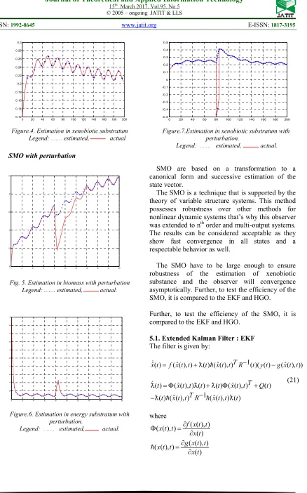
Figure.4. Estimation in xenobiotic substratum

Legend: ... estimated, actual

SMO with perturbation

0 20 40 60 80 100 120 140 160 180 200 0.5

[image:7.612.113.273.292.427.2]

0.55 0.6 0.65 0.7 0.75

Fig. 5. Estimation in biomass with perturbation Legend: ... estimated, actual.

0 20 40 60 80 100 120 140 160 180 200 0

0.05 0.1 0.15 0.2 0.25 0.3 0.35 0.4 0.45 0.5

Figure.6. Estimation in energy substratum with perturbation.

Legend: ... estimated, actual.

0 20 40 60 80 100 120 140 160 180 200

-0.5 -0.4 -0.3 -0.2 -0.1 0 0.1 0.2 0.3 0.4 0.5

Figure.7.Estimation in xenobiotic substratum with perturbation.

Legend: ... estimated, actual.

SMO are based on a transformation to a canonical form and successive estimation of the state vector.

The SMO is a technique that is supported by the theory of variable structure systems. This method possesses robustness over other methods for nonlinear dynamic systems that’s why this observer was extended to nth order and multi-output systems. The results can be considered acceptable as they show fast convergence in all states and a respectable behavior as well.

The SMO have to be large enough to ensure robustness of the estimation of xenobiotic substance and the observer will convergence asymptotically. Further, to test the efficiency of the SMO, it is compared to the EKF and HGO.

Further, to test the efficiency of the SMO, it is compared to the EKF and HGO.

5.1. Extended Kalman Filter : EKF The filter is given by:

1

ˆ( ) ( ( ), )ˆ ( ) ( ( ), )ˆ T ( )( ( ) ( ( ), ))ˆ

x t& = f x t t +D t h x t t R− t y t −g x t t

ˆ ˆ

( ) ( ( ), ) ( ) ( ) ( ( ), ) ( ) 1

ˆ ˆ

( ) ( ( ), ) ( ( ), ) ( )

T t x t t t t x t t Q t

T

t x t t R x t t t

= Φ + Φ +

− −

&

D D D

D h h D

where

( ( ), ) ( ( ), )

( ) ( ( ), ) ( ( ), )

( )

f x t t x t t

x t g x t t x t t

x t

∂

Φ =

∂ ∂ =

∂

h

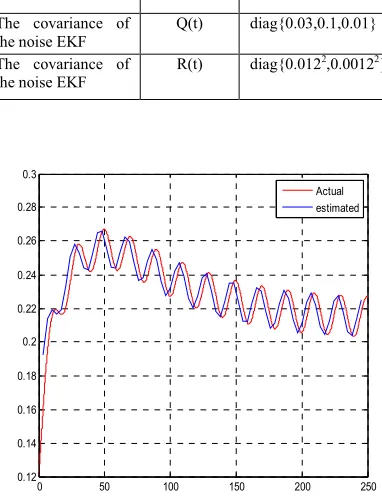
The results obtained by applying the EKF were obtained with the numerical values of the parameters of synthetic data in the table 2[18].

TABLE 2:SYNTHESIS PARAMETERS OF THE EKF

Description Parameters Values The covariance of

the noise EKF

Q(t) diag{0.03,0.1,0.01} The covariance of

the noise EKF

R(t) diag{0.0122_,0.00122_}

0 50 100 150 200 250 0.12

0.14 0.16 0.18 0.2 0.22 0.24 0.26 0.28 0.3

[image:8.612.98.289.166.415.2]

Actual estimated

Figure. 8. Estimation in xenobiotic substratum

The EKF observer provides recursive optimal state estimation for the system of waste water treatment but it’s not very efficient and so the robustness and precision are reduced. For application of this observer, there is a lag (error of estimation is very large;x%= −xˆ x_{) between the real substratum and}

its estimate.

5.2. High gain observer structure

For general nonlinear system, a high gain observer is used to handle part of the nonlinearity of the system by choosing a sufficiently large value of a given design parameter [19].

The system is written on the following form: ( , )

1 1

2

x F u x x

y Cx x

x



 _{ }

 _{ }

 _{ }

  



=

= = =

&

2

( ) ; ; ( )

1 1 2 3 1

avec 1 1 2

T

x x x x x D t u q

p n n n_q n n k k

= = =

= ≥ ≥L≥ _{∑ =} =

So, 2 1 2

1 2

p=n = ≥n = → =q

We have xk∈Rnk;k=1,...,q

as a result 1x ∈Rn1=R2 and x2∈Rn2=R1

The proposed observer is the following one:

1 1 1

ˆ ( , )ˆ ( , )ˆ T ; ˆ

x&=F u x −ψδ+ u x ∆_ψ− −γ C Cx x% %= −x x

( , )u x

δ is left invertible (assumption (A1)),

( , )u x

δ

+ its left inverse.γ ,∆

_ψ

, Cand

δ

+( , )u xˆ are given above.

0 20 40 60 80 100 120 140 160 180 200 0.12

0.14 0.16 0.18 0.2 0.22 0.24 0.26 0.28 0.3

Figure.9. Estimation in xenobiotic substratum Legend: ... estimated, actual.

Simulation results carried out a system of waste water treatment have been reported. These simulations showed the good capabilities of the designed high gain observer in providing good estimates for the non-measurable states. High gain observer addressed is a suitable nonlinear observer which can estimate non-measurable states.

The simulation results confirm that HGO and SMO have stronger parameter ability than the EKF. So, we can consider that SMO and HGO, compared to EKF, are the main solution to the system in order to increase its robustness and improve dynamic performance. But we can see that SMO can have more effectiveness than HGO and to confirm this, we have done a comparative study more precious.

The experimental evaluation of the HGO and SMO is shown as regards:

*Observer performance and the mean square error, *Sensitivity to perturbation and noise measure, *Convergence and algorithm complexity… (22)

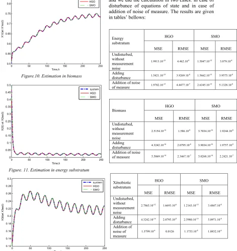
[image:8.612.332.533.295.449.2]

6. COMPARATIVESTUDY:SMO AND HGO

Following the simulation using the new technique (SMO) to that studied (HGO), the estimation in biomass is presented in figure (10), whereas the estimation in energy substratum is viewed in figure (11) and the estimation in xenobiotic substratum is displayed in figure (12).

0 50 100 150 200 250

0.5 0.55 0.6 0.65 0.7 0.75 0.8 0.85

Time,h

X

1

(t

)e

t

X

1

e

s

(t

)

[image:9.612.97.568.203.703.2]

system HGO SMO

Figure.10. Estimation in biomass

0 50 100 150 200 250 0

0.05 0.1 0.15 0.2 0.25 0.3 0.35 0.4 0.45 0.5

Time,h

X

2

(t

)

e

t

X

2

e

s

(t

)

system HGO SMO

Figure. 11. Estimation in energy substratum

0 50 100 150 200 250

0.12 0.14 0.16 0.18 0.2 0.22 0.24 0.26 0.28 0.3

Time,h

X

3

(t

)e

t

X

3

e

s

(t

)

system HGO SMO

Figure.12. Estimation in xenobiotic substratum

The Mean Square Error (MSE Mean Square Error) is the arithmetic mean of the squared differences between forecasts and observations. However, RMSE is the Root Mean Square Error.

In this section, we will look at a more accurate and precise comparison of the SMO and HGO to show the best. For this, we proceeded to make a summary table containing the values of the MSE and RMSE and we did the calculation in two cases: in case of disturbance of equations of state and in case of addition of noise of measure. The results are given in tables’ bellows:

Energy substratum

HGO SMO

MSE RMSE MSE RMSE

Undisturbed, without measurement noise

1.9913.10-15 _4.462.10-8 _1.5047.10-15 _3.879.10-8

Adding

disturbance 1.5421.10 -15

3.9269.10-8

1.5662.10-15

3.9575.10-8

Addition of noise

of measure 1.9782.10 -13

4.4477.10-7

2.6345.10-15

5.1328.10-8

Biomass

HGO SMO

MSE RMSE MSE RMSE

Undisturbed, without measurement noise

2.5154.10-16

1.586.10-8

3.7034.10-16

1.9244.10-8

Adding

disturbance 4.3242.10 -16

2.0795.10-8

3.9034.10-16

1.9757.10-8

Addition of noise

of measure 5.5069.10-14 _2.3467.10-7 _5.0268.10-14 _2.2421.10-7

Xénobiotic substratum

HGO SMO

MSE RMSE MSE RMSE

Undisturbed, without measurement noise

2.7865.10-12 _1.6693.10-6 _1.2143.10-15 _3.4847.10-8

Adding

disturbance 4.3242.10

-16 _2.0795.10-8 _2.5980.10-15 _5.0971.10-8

Addition of noise of measure

1.5799.10-4

0.0126 1.1733.10-8

COMMENT

The nonlinear observers that we presented all show their ability to reconstruct the evolution of the concentration of elements biochemical. Given the strong nonlinearity characterizing the dynamics of pollution control process (degradation bi-substratum, coupling due to the inhibition / activation), we can be satisfied with the behavior of these observers. But, some comparative remarks are necessary.

We see that the convergence of SMO is fast enough, it was more a good estimate of the variable

( )

s_x t compared to the results for the previous two observers (especially EKF), the evolution of the estimated values of the concentration of substrates

( )

c t

b , e tn( ) and sx( )t has a relatively smooth

appearance.

The SMO has shown a good ability to reconstruct the xenobiotic substratum concentration (we're going to regulate) and that assuring a low square error compared to that of HGO in the case of disturbance of state equations or adding noise of measure.

The convergence of both observers SMO and HGO is very satisfactory compared to the EKF. In fact, the speed of the estimated variables is relatively smooth compared to the previous observer (EKF).

The energy substratum being measured, the influence ofs_x( )t through its filtered value is

negligible due to the weak inhibition of η_e( )t by

the substratums_x( )t . In conclusion, we can notice that the SMO has very good capacity of filtering of noise of measure.

7. CONCLUSION

In this paper, a sliding mode observer for a class of nonlinear systems in a special canonical observable form was proposed and it was compared with EKF and HGO.

This observer provides a good solution to estimate state parameters in the studied biochemical system. The obtained simulation results show good performances.

The implementation of the EKF involves significant numerical complexity compared to the SMO and HGO.

As an estimator for the states of system of waste water treatment, the Kalman filter does not perform as well as the HGO and the SMO. Also, SMO is very efficient than HGO because it gives most important results. The robustness of the SMO is more guaranteed. The sensitivity to addition noise of measure and perturbation are also guaranteed.

Finally, the SMO is considered the most convenient one compared to the EKF and HGO. It is more available and much simpler to implement in order that the dynamic performances can be more guaranteed.

REFRENCES:

[1] J.P.Gauthier,H.Hammouri and S.Othman, “A

simple observer for nonlinear systems

applications to bioreactors”, IEEE

Trans.Autom.Control, vol.37,No.6, 1992, pp.875-880.

[2] F.Deza, E.Busvelle,J.P.Gauthier and

D.Rakotopara, “high gain estimation for nonlinear system”, Syst.Control let.,vol.18, No.4, 1992, pp.295-299.

[3] F.Deza,D.Boussanne, E.Busvelle, J.P.Gauthier

and D.Rakotopara, “Exponential observers for

nonlinear systems”, IEEE

Trans.Autom.Control,vol.38,No.3,1993, pp.482-484.

[4] K.Busawon, M.Farza, and H.Hammouri,

”Observer design for a special class of nonlinear

systems”, Int.J.Control,vol.71,No.3,1998,

pp.405-418.

[5] H.Gouta, S.HadjSaid, N.Barhoumi and F.M'Sah

li, “Observer Based Backstepping controller for

a state coupled two tank system”, IETE Journal

of Research, Vol. 61, No 3, 2015, pp 259-268.

[6] K. Vijayaraghavan,” Nonlinear Observer for

simultaneous states and unknown parameter estimation”, IETE Journal of Research, Vol.86, No. 12, 2013, pp.2263-2273.

[7] J.Aslund and E.Frisk,” Observers for non-linear

differential-algebraic systems”, Department of Electrical Engineering, Linköping University, 2012, 581 83.

[8] J.Gonzalez,G.Fernandez,R.Aguilar,M.Barron

and J.Alvarez-Ramirez, “Sliding mode

observer-based control for a class of

bioreactors”,Chemical Engineering Journal

Vol.83, 2000, pp.25-32.

[9] H.K.Kim, T.T.Nguyen and S.B.Kim,”Nonlinear

Process in Stirred Tank Bioreactor”, ICASE: The Institute of control, Automation, and Systems Engineers,KOREA Vol.4,No.3, 2002.

[10] M.Farza,K.Busawon and H.Hammouri,”Simple

nonlinear observers for on-line estimation of

kinetic rates in bioreactors”, Automatica

,Vol.34,No.3,1998, pp.301-318.

[11]M.Farza,H.Hammouri,C.Jallut and

J.Lieto,”State observation of a nonlinear system: application to bio chemical process”,

AIChE J. Vol.45No.1,1999, pp.93-106.

[12]P.P.Biswas, S.Ray and A.N.Samanta,

“Multi-objective constraint optimizing IOL control of distillation column with nonlinear observer,”,

Journal of Process Control Vol.17, 2007, pp. 73-81.

[13]M.Farza, M.M’Saad and M. Sekher. “A set of observer for a class of nonlinear systems”, 2005.

[14]Q.chai. “Modeling, estimation and control of biological wastewater treatement plants”, Thesis presented in NTNU,april 5,2008.

[15]H.Hammouri and M. Farza. “Nonlinear

observers for locally uniformly observable systems”, ESAIM J. on Control, Optimisation and Calculus of Variations, Vol. 9,2003, pp. 353–370.

[16]S.hadj Said and F.M’Sahli.”A Set of Observers

Design to a Quadruple Tank Process”, 17th

IEEE International Conference on Control Applications Part of 2008 IEEE Multi-conference on Systems and Control San Antonio, Texas, USA, September 3-5, 2008.

[17]M.Farza,H.Hammouri,C.Jalfut and

J.Lieto,”State observation of nonlinear system: application to biochemical process”, AIChE J.

Vol.45,1998b.

[18]A.Barhoumi,T.Ladhari and F.M’Sahli,” The

extended Kalman Filter For Nonlinear

System:Application to System of Waste water

Treatment”, STA’14,Tunisie, December 2014.

[19]A.Barhoumi,T.Ladhari and F.M’Sahli, ”High

Gain Observer For Nonlinear System:

Application to System of Waste water

Treatment”, SSD’15,Tunisie, March 2015.

[20]H.Nijmeijer and T.Fossen, ”New Directions in Nonlinear Observer Design”. Springer: Berlin, 1999.

[21]L.Fridman, Y.Shtessel, C.Edwards and

X.G.Yan,”Higher-order sliding-mode observer for state estimation and input reconstruction in nonlinear systems”, International Journal Of Robust And Nonlinear Control, March 2008.

[22]C.Yang,Q.kong and Q.Zhang,”Observer design

for a class of nonlinear descriptor systems”,

Journal of the Franklin Institute,vol.350, No.5, june 2013.

[23]R.A.Farshbaf, M.R.Azizian, K.Amiri and

M.J.Khosrowjerdi,”A Comparative Study of Speed Observers between Adaptive and Sliding

Mode Approaches”, The 5th Power

Electronics, Drive Systems and Technologies Conference (PEDSTC 2014), Tehran, Iran, Feb 5-6, 2014.

[24]C.Ben Youssef and B.Dahhou.”Multivariable

adaptive control and estimation of nonlinear wastewater treatment process” , Proceeding of the 3rd IEEE Mediterranean Symposium on New Directions in Control and Autmation,Limassol,Chypre,1,1995, pp.220-224.

[25] P. Vigie, B. Dahhou, I. Queinnec, M. Lakrori, A. Cheruy and J.B. Pourciel. “Control of

substrate concentration in a continuous

bioprocess”, Bioprocess Engineering, vol.6,

No.6, 1991, pp.259-263.

[26]S.Ammar and M.Mabrouk,,” Observer and

output feedback stabilisation for a class

of nonlinear systems”, IETE Journal of

Research, Vol. 83, No. 5, 2010, pp 983-995.

[27]K.C. Veluvolu, M.Y. Kim and D.

Lee,”Noninear sliding mode high-gain