Research on the Portfolio Optimization Model under Quantitative Constraint Based on Genetic Algorithm

(1)

ISSN Online: 2162-2442 ISSN Print: 2162-2434

DOI: 10.4236/jmf.2016.64037 September 16, 2016

Research on the Portfolio Optimization Model

under Quantitative Constraint Based on

Genetic Algorithm

*

Shunquan Zhu

School of Finance, Guangdong University of Finance & Economics, Guangzhou, China

Abstract

This paper is based on covariance and expected return, building portfolio risk opti-mization model. Using Genetic Algorithm and Quadratic Programming, three secur-ities portfolio Optimization model is resolved, and we find that Genetic Algorithm having priority for Restraint Conditions is not a linear model.

Keywords

Portfolio Optimization Decision Making, Quadratic Programming, Genetic Algorithm

1. Background

The number of securities transactions is generally limited in the capital market. For example, the minimum number of regular trading stocks is 100 shares, and trading less than 100 shares is not accepted in Shanghai Stock Exchange and Shenzhen Stock Ex-change. On the other hand, for various considerations, investment institutions and in-vestors often set certain requirements for funds allocation, and portfolio needs to meet these requirements. In order to adapt the need for capital market and practical opera-tion, it is necessary to research portfolio decision problem under risk constraint. But it is difficult to express the portfolio optimization model under numeric constraint from existing literature [1]-[5].

Genetic algorithm is based on the mechanism of natural selection and evolution. For

*This paper is supported by Guangdong Provincial Scientific Plan Project (Soft Science, No.: 2015-A070704058), Guangdong Provincial Universities’ Social Science Fund Project (No.: 2015WTSCX031), The Natural Science Foundation of Guangdong (No.: 2015A030313629), The Graduate Student Education Innovation Projects in Guangdong (No. 2-2015), and the National Natural Science Foundation of China.

How to cite this paper: Zhu, S.Q. (2016) Research on the Portfolio Optimization Mod-el under Quantitative Constraint Based on Genetic Algorithm. Journal of Mathemati-cal Finance, 6, 465-470.

http://dx.doi.org/10.4236/jmf.2016.64037

Received: June 12, 2016 Accepted: September 13, 2016 Published: September 16, 2016

(2)

almost 30 years of research and application, genetic algorithm is now widely used in optimization function, neural network learning procession, pattern recognition, indus-trial process control system and other fields. However, it is still not common to solve portfolio optimization problem under numeric constraint by genetic algorithm. This paper attempts to use genetic algorithm to solve this problem, and in order to verify the reliability of this method, a function with quadratic programming in Matlab to calcu-late the results is used.

2. Build the Portfolio Optimization Model under Numeric

Constraint [6]

Consider investment institution (e.g. Fund Company) or investors invest in n kinds of risky assets. We denote the expected returns and portfolio weights of risky assets by the vectors R=

(

r r1, ,2,rn

)

′, x=

(

x x1, 2,,xn

)

′. The variance-covariance matrix of the

risky assets’ returns matrix is V =

( )

σij _{n n}_× , it is positive definite. L=

(

l l1, ,2 ,ln

)

′,

(

1, 2, , n

)

U = u u  u ′ represents all components of the column vector, li∈

( )

0,1 ,ui∈

( )

0,1 .

(

1,1, ,1

)

l=  ′ represents all components of the column vector is 1. The efficient

port-folio decision model under number constraint is denoted by

( )

2

Min

σ

x =x Vx′

s.t. R x′ ≥µ,l x′ =1,L≤ ≤x U.

However, it is difficult to obtain the optimal analytical expression for this problem, so we try to solve this problem by genetic algorithms.

3. Use Genetic Algorithms to Solve Portfolio Decision Model

under Numeric Constraint [7]

3.1. Initialization

1) Determine population size M, crossover probability pc, mutation probability pm, maximum evolution generation maxgen, the vector of upper and lower bounds

(

1, ,2 ,n

)

L= l l  l ′, U =

(

u u1, 2,,un

)

′, li∈

( )

0,1 ,ui∈

( )

0,1 .

2) Use real-code, each chromosome contains n gene loci which represent insecurities, the genevaluation represents the proportion in securities portfolio.

3) It is easy to know the following super geometry contains feasible set from the con-straints. Consider x1′

( )

0 =u

( ) ( )

0,1 ,x2′ 0 =u

( )

0,1 ,,xn′

( )

0 =u

( )

0,1 , where U(0,1) re-

presents a random number that should be uniformly distributed between (0,1), then normalize x′j

( )

0 denoted by

( )

1

0 0 0

n

j j j

j

x x x

=

′ ′

=

∑

_{, and} x

( )

0 =

(

x1

( )

0 ,,xn

( )

0

)

.

If the result does not satisfy the constraint, reject it. Then we need to use the third step to generate a new chromosome, if the chromosome is feasible, we can accept it as a member of population, then we use the notation xj,j=1, 2,,M to denote M

feasi-ble chromosome after finite sampling. Consider the code of x is v, and denoted by

( )

0

(

1

( )

0 , , M

( )

0 .

)

v = v  v

(3)

( )

(

)

2

(

( )

)

0 0

j j

F v = −σ v . It is better to reorder the vj

( )

0 according to the target value,

and denote the first row chromosome as v0. If we find a better chromosome in the

fu-ture evolution, use this and replace v0.

5) Set k = 0.

3.2. Selection

1) According to the principle that the more adaptable the chromosomes are, the more chance they would be selected to reproduce. Breeding probabilities for each

( )

j

v k are based on the adaptability

( )

(

( )

)

( )

(

1

)

(

2

( )

)

(

( )

)

.

j j

n

F v k

p k

F v k F v k F v k

=

+ + +_

j = 1means that the chromosome is the best, j = M explains the chromosome is the worst.

2) Calculate the cumulative probability vj

( )

k for each chromosome.

( )

0

1

0, , 1, 2, , .

j

j i

i

q q p k j M

=

= =

∑

= _

3) Generate a random number r in

(

0,qM

)

. If qj−1< <r qj chose the jth

chromo-some. 1≤ ≤j M

4) Repeat step 2 and 3 for m times in total, then we can obtain m replicated chromo-somes denoted by v′=

(

v k1′

( )

,,v′M

( )

k

)

.

3.3. Hybridization

1) Define pc as the probability of hybridization in advance, v′j

( )

k is the parent of

hybridization. Repeat the following step from j = 1 to M: Generate a random number denoted by r in [0, 1]. Chose v′j

( )

k as a parent if r< pc.

2) We use the notation v k1′′

( )

,,vL′′

( )

k to denote the parents, and group them

randomly such as

(

v k1′′

( )

,,vL′′

( )

k

)

, hybridization is performed on all groups. To

perform the operation on

(

v k1′′

( ) ( )

,v2′′ k

)

, generate a random number c from (0,1)

firstly, and then perform the hybridization as the following form between

(

v k1′′

( ) ( )

,v2′′ k

)

to produce two offspring:

( )

( ) (

) ( )

1 1 1 2

x k =cv k′′ + −c v′′ k ; x2

( ) (

k = −1 c v k

) ( )

1′′ +cv2′′

( )

k .

3) We can use hybridization on the other group as the same way.

3.4. Mutation

1) First, define the mutation probability pm. For the individuals through crossover operation mutate from j = 1 to M, repeat the following step: generate a random number r from [0,1], if r< pm, select it as mutation parent.

(4)

on the chromosome aij. If the constraints are not satisfied, refuse the result. Follow step 2 to generate a new chromosome, if this one is feasible, accept it as a population mem-ber. It will generate s new mutated individuals after finite sampling.

3) Consider s new individuals by mutation operation and L-s new individuals that are not selected from hybridization in step 2, calculate their valuation. And then put them back simultaneously. There are M-L remaining individuals by choosing operation. All of them consist of a new generation denoted by v k

(

+ =1

)

{

v k1

(

+1 ,

)

,vM

(

k+1

)

}

.

4) Termination test

If reach the maximum number of evolution, evolution is terminated, otherwise set

k = k + 1, turn to the selection operation.

4. The Example of the Risk on Optimal Portfolio by Genetic

Algorithms and Analysis

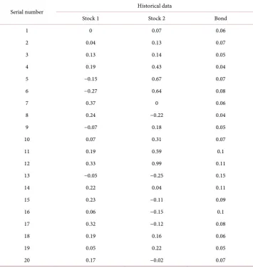
[image:4.595.196.552.330.707.2]

Obtain three monthly securities’ returns from financial database [8] by downloading and sorting (as shown in Table 1).

Table 1. Historical data of returns for three securities.

Serial number Historical data

Stock 1 Stock 2 Bond

1 0 0.07 0.06

2 0.04 0.13 0.07

3 0.13 0.14 0.05

4 0.19 0.43 0.04

5 −0.15 0.67 0.07

6 −0.27 0.64 0.08

7 0.37 0 0.06

8 0.24 −0.22 0.04

9 −0.07 0.18 0.05

10 0.07 0.31 0.07

11 0.19 0.59 0.1

12 0.33 0.99 0.11

13 −0.05 −0.25 0.15

14 0.22 0.04 0.11

15 0.23 −0.11 0.09

16 0.06 −0.15 0.1

17 0.32 −0.12 0.08

18 0.19 0.16 0.06

19 0.05 0.22 0.05

(5)

Calculate covariance matrix for three securities with function corvar() in Excel

0.052122 0.02046 0.00025

0.02046 0.20929 0.00023 .

0.00025 0.00023 0.00147

V

− −

 

 

= −_ − _

− − 

 

Calculate expected return on three securities, denoted by R, with function average,

(

0.1130, 0.1850, 0.0755

)

R= .

Consider the minimum expected return on the three securities is 0.13, calculate the optimal proportion and lowest risk under the condition of no short sale.

We use genetic function GA in Matlab, the program is as follows. The M file by Genetic Algorithm denoted by tzga.m

Obj = @tzfitness;

Nvars = 3; % Number of variables A = [−0.1130, −0.1850, −0.0755]; b = [−0.13]; Aeq = [1,1,1]; beq = [1]; LB = [0 0 0]; % Lower bound UB = [1 1 1]; % Upper bound

% Constraint Function = @tzconstraint; [x,fval] = ga(Obj,nvars,A,b,Aeq,beq,LB,UB,[])

The function by genetic algorithm denoted by tzfitness.m function y =tzfitness(x)

( ) ( )

( )

( ) ( )

( )

0.

02610 * 1 * 1 0.104645* 2 * 2 0.0007345* 3 * 3 0.02046 * 1 * 2 0.00025* 1 * 3 0.00023* 2 * 3 ;

y x x x x x x

x x x x x x

= + +

− − −

The results are running as the above program in Matlab as follows: >> tzga

x = 0.5044 0.3245 0.1718 fval = 0.0143

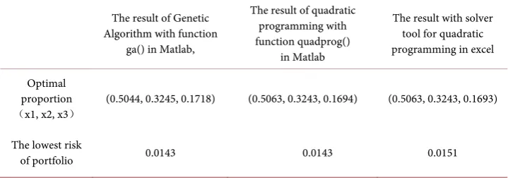
[image:5.595.193.553.581.707.2]

Compare the above results and the results get by quadratic programming with Mat-lab function quadprog() [9] and Excel Solver tool, calculate them and show them in

Table 2.

As shown in Table 2, the results of Portfolio Optimization Model with three me-thods are close. But the function qudprog() in Matlab and solver tool in excel are only

Table 2. Results of calculation of the three methods.

The result of Genetic Algorithm with function

ga() in Matlab,

The result of quadratic programming with function quadprog()

in Matlab

The result with solver tool for quadratic programming in excel

Optimal proportion （_{x1, x2, x3}）

(0.5044, 0.3245, 0.1718) (0.5063, 0.3243, 0.1694) (0.5063, 0.3243, 0.1693)

The lowest risk

(6)

adapted to linear and quadratic programming model. In addition to Quadratic Pro-gramming under liner, genetic algorithm can solve quadratic proPro-gramming under non-linear constraint, even to the complex model in which the objective function is a Non-linear model that is not quadratic programming and the constraint is nonNon-linear, genetic algorithm also can solve it. Therefore, the advantages of genetic algorithms are incom-parable in modeling complex social and economic life.

5. Overview

In order to make the portfolio optimization problems close to reality, we often need to study the portfolio optimization problem under numeric constraint. This paper is based on this model to calculate the optimal portion by code; selection, crossover and muta-tion are adapted to portfolio decisions successfully, and optimal solumuta-tion can be ob-tained. In order to prove the reliability of the genetic algorithm, we use quadratic pro-gramming with function quadprog() in Matlab and solver tool for quadratic program-ming in excel to solve this problem. This paper shows that the genetic algorithm is bet-ter than quadratic programming, because the genetic algorithm can solve non-quadratic programming problems. It is foreseeable that in the future genetic algorithms will be used widely for practical application in portfolio optimization.

References

[1] Markowitz, H. (1952) Portfolio Selection. Journal of Finance, 7, 77-91.

http://dx.doi.org/10.1111/j.1540-6261.1952.tb01525.x

[2] Sharpe, W.F. (1963) A Simplified Model for Portfolio Analysis. Management Science, 1, 277-293. http://dx.doi.org/10.1287/mnsc.9.2.277

[3] Sharpe, W.F. (1967) A Linear Programming Algorithm for Mutual Fund Portfolio Selection.

Management Science, 3, 499-510. http://dx.doi.org/10.1287/mnsc.13.7.499

[4] Sharpe, W.F. (1967) A Portfolio Analysis. Journal of Finance and Quantitative Analysis, 6, 76-84.

[5] Zhu, S.Q. (2012) Investment. Theory. Application. Experiment. Tsinghua University Press, Beijing, 1.

[6] Zhang, W.G. (2007) Modern Portfolio Theory—Model, Methods and Application. Science Press, Beijing, 3.

[7] Lin, D. (2005) Improved Portfolio Investment Model with Genetic Algorithm. Systems En-gineering, 8, 68-72.

[8] Zhu, S.W. (2007) Financial Database. Tsinghua University Press, Beijing, 12.

(7)

Submit or recommend next manuscript to SCIRP and we will provide best service for you:

Accepting pre-submission inquiries through Email, Facebook, LinkedIn, Twitter, etc. A wide selection of journals (inclusive of 9 subjects, more than 200 journals)

Providing 24-hour high-quality service User-friendly online submission system Fair and swift peer-review system

Efficient typesetting and proofreading procedure

Display of the result of downloads and visits, as well as the number of cited articles Maximum dissemination of your research work