Geophysicae
The estimation of D-region electron densities from riometer data
J. K. Hargreaves1and M. Friedrich2
1Department of Communication Systems, University of Lancaster, Lancaster, UK
2Department of Communications and Wave Propagation, Technical University of Graz, Graz, Austria
Received: 7 March 2002 – Revised: 3 July 2002 – Accepted: 23 August 2002
Abstract. At high latitude the hard electron precipitation as-sociated with auroral activity is a major source of ionization for the D-region, one consequence being the absorption of radio waves. Direct measurements of the D-region electron density are not readily available, however. This paper inves-tigates the relationship between the electron density at alti-tudes between 100 and 70 km and the total radio absorption observed with a riometer, with a view to using the latter to predict the former. Tables are given of the median electron density corresponding to 1 dB absorption at 27.6 MHz for each hour of the day, and it is shown that at certain heights the estimates will be accurate to within a factor of 1.6 on 50% of the occasions. A systematic variation with time of day is probably associated with a progressive hardening of the typ-ical electron spectrum during the morning hours. There is also evidence for a seasonal effect possibly due to seasonal variations of the mesosphere.
Key words. Ionosphere (auroral ionosphere) – Radio sci-ence (ionospheric propagation; instruments and techniques)
1 Introduction
In the auroral regions the principal source of D-region ion-ization is the flux of energetic electrons during auroral ac-tivity. There are, of course, contributions from other sources, such as solar electromagnetic emissions (particularly Lyman-αand X-rays), and these are enhanced during solar flares. Solar protons cause ionization down to relatively low alti-tudes during solar proton events, but such events are much less frequent than auroral precipitation. Overall, the electron flux at energies from a few tens of keV to a few hundred keV may be assumed to be the dominant source most of the time, contributions from other ionization sources being generally less significant.
Direct observations in the D-region may be made by rocket-borne instruments, and although these techniques are Correspondence to: J. K. Hargreaves
well established (Mechtly, 1974; Jacobsen and Friedrich, 1979), they are expensive and the data are limited because each flight produces only a single profile. Since the mid 1970s, and more particularly, since the EISCAT system be-gan to operate in the early 1980s, it has been possible to mea-sure electron densities in the D-region by incoherent scatter radar (Hunsucker, 1974; Ranta et al., 1985; Devlin et al., 1986). Under good conditions it is possible to obtain accurate measurements at 1 km height resolution and 10 s time reso-lution. Radar is considerably less sensitive than the rocket-borne probes but it may provide continuous runs of data over several hours. However, the radar data are still limited be-cause incoherent scatter radars are few in number and immo-bile, and they are also expensive to operate.
Another way of detecting enhancements in the D-region is by measuring the absorption of a radio signal that has passed through the medium. This is the purpose of the riometer tech-nique in which the intensity of the cosmic radio noise at some frequency, usually between 20 and 60 MHz, is monitored us-ing a stable receiver at the ground (Hargreaves, 1969). The riometer is relatively cheap and simple to operate. Many of them have been, and still are, in use.
This paper addresses the question of whether riometer data may realistically be used to indicate the electron density at a selected altitude. The depth to which an incoming electron penetrates into the atmosphere depends on its initial energy (Rees, 1963), the more energetic ones depositing their en-ergy at lower altitudes. The resulting electron-density pro-file, therefore, depends on the original spectrum of the in-cident particles. Then, if the electron density isNe(h), the
absorption of a radio wave of angular frequencyω=2πf is
A (dB)=4.6×10⁻⁵
Z N
e(h)ν(h)
ω2+ν(h)2dh , (1)
(Hargreaves, 1969) whereν(h) is the electron-neutral colli-sion frequency. Whileν(h) is a property of the atmosphere (i.e. proportional to pressure),Ne(h)depends on the
rela-(a)
(b)
Fig. 1. (a) Value of 90 km electron density corresponding to 1 dB absorption for the whole data set between 1985 and 1992. (b) Distribution of data points with month and time of day.
tionship between radio absorption and electron density. But neither is the spectrum entirely random. Therefore, we may reasonably ask to what extent, if any, ground-based absorp-tion measurements may be used to indicate D-region elec-tron density, and, if so, what will be the accuracy of these estimates.
2 The present investigation and data used
Friedrich and Kirkwood (2000) have published average electron-density profiles corresponding to selected absorp-tion levels. Most of the data came from EISCAT for the
(a)
(b)
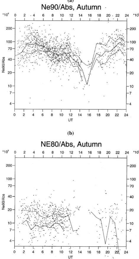
Fig. 2. Values ofNe/A against time of day for (a) 90 km and
(b) 80 km.
greater heights and from rockets for the lower ones below about 80 km. The profiles were divided according to whether or not the D-region was illuminated by the Sun. The present study seeks to extend those results in two directions: by spec-ifying the likely accuracy of the estimates, and by looking at the change from night to day in greater detail.
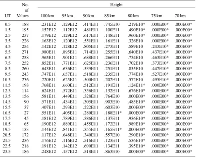
[image:2.595.52.285.66.515.2] [image:2.595.311.547.69.508.2]Table 1. Median electron density corresponding to 1 dB absorption for each height and each hour of the day, using data from all years and months. The * indicates an upper quartile
No. Height
of
UT Values 100 km 95 km 90 km 85 km 80 km 75 km 70 km
0.5 188 .231E12 .129E12 .414E11 .745E10 .219E10* .000E00* .000E00* 1.5 195 .152E12 .112E12 .481E11 .100E11 .490E10* .000E00* .000E00* 2.5 237 .179E12 .129E12 .617E11 .148E11 .960E10* .000E00* .000E00* 3.5 226 .163E12 .120E12 .551E11 .161E11 .326E10 .000E00* .000E00* 4.5 254 .142E12 .128E12 .805E11 .273E11 .589E10 .243E10* .000E00* 5.5 271 .980E11 .895E11 .714E11 .255E11 .640E10 .437E10* .000E00* 6.5 258 .965E11 .901E11 .688E11 .266E11 .734E10 .463E10* .000E00* 7.5 252 .852E11 .771E11 .625E11 .236E11 .702E10 .373E10* .000E00* 8.5 260 .643E11 .636E11 .539E11 .251E11 .855E10 .447E10* .000E00* 9.5 243 .747E11 .657E11 .518E11 .235E11 .774E10 .527E10* .000E00* 10.5 236 .720E11 .625E11 .500E11 .202E11 .572E10 .495E10* .000E00* 11.5 198 .768E11 .660E11 .512E11 .191E11 .124E11* .000E00* .000E00* 12.5 114 .624E11 .572E11 .356E11 .132E11 .676E10* .000E00* .000E00* 13.5 156 .581E11 .449E11 .328E11 .764E10 .000E00* .000E00* .000E00* 14.5 90 .571E11 .434E11 .305E11 .903E10 .485E10* .000E00* .000E00* 15.5 37 .407E11 .293E11 .222E11 .603E10 .000E00* .000E00* .000E00* 16.5 27 .551E11 .405E11 .280E11 .188E11* .000E00* .000E00* .000E00* 17.5 45 .181E12 .789E11 .386E11 .137E11 .936E10* .000E00* .000E00* 18.5 65 .190E12 .889E11 .455E11 .172E11 .989E10* .000E00* .000E00* 19.5 133 .144E12 .841E11 .355E11 .165E11* .000E00* .000E00* .000E00* 20.5 172 .117E12 .648E11 .340E11 .557E10 .290E10* .000E00* .000E00* 21.5 236 .176E12 .116E12 .516E11 .123E11 .536E10* .000E00* .000E00* 22.5 218 .191E12 .142E12 .690E11 .134E11 .395E10* .000E00* .000E00* 23.5 186 .248E12 .157E12 .518E11 .863E10 .000E00* .000E00* .000E00*
site at Ramfjordmoen, Norway (69.6◦N, 19.2◦E,L =6.2), specifically two each at Ramfjordmoen and at Lavangsdalen. The absorption values are converted to 27.6 MHz, X-mode and vertical incidence (Friedrich et al., 2002). Both data sets are at a 5-min interval. Since the riometer data are relatively less accurate at small values, and to reduce the effect of solar contributions to the absorption (which could amount to a few tenths of a dB at noon), only values of at least 0.5 dB are used in the following analysis.
3 Data analysis
Since the absorption at a given height is proportional to the electron density (Eq. 1), we work with the ratioNe(h)/A,
whereNe(h)is the electron density in m−3at heighthand
Ais the total absorption at 27.6 MHz in dB. Figure 1a shows the values ofNe(90)/Aover the whole data set against the
year. Its value spreads by about a factor of 10, but there is no indication of a systematic variation from year to year. We shall, therefore, take all the years together. Figure 1b shows the distribution of data points with month and time of day. This distribution is less even than we might wish. The gap in the afternoon corresponds with the low occurrence of auroral absorption at that time of day, which is well known
(Harg-reaves and Cowley, 1967), but the gaps during the summer period, and during the winter, from Christmas to the end of January, are plainly observational and due to the schedules of radar operations.
As an example of the results, Fig. 2 shows the values of Ne/Afor 90 and 80 km for the autumn period (months 8.25–
11.25) against time of day, with medians and quartiles super-imposed. At 90 km there is a marked variation with time of day, particularly during the morning hours. That variation is not apparent at 80 km. In that case, however, medians were obtained only for the hours 01:00 to 11:00 UT. At other times only the upper quartiles are shown. The lower quartiles are lost in the zeros of the data set, and are not plotted; they fall below the limit of measurement.
Table 1 summarizes the median values of electron den-sity corresponding to 1 dB absorption for each hour of the UT day. When no median was obtained, the upper quartile is marked with an asterisk. This table uses the values from all months. The relative lack of data in summer and winter makes it more difficult to look for seasonal variations, but we will return to this point in a later section.
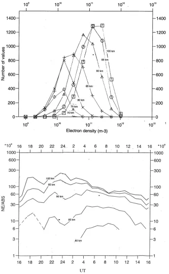
Fig. 3. Histograms of electron density from 100 km to 70 km.
[image:4.595.45.379.60.600.2]UT
Fig. 4. Medians for whole data set, 1985–1992. Variation of median elec-tron density (for 1 dB absorption) with time of day. At EISCAT local mag-netic midnight is about 21:30 UT. The data show a daily cycle starting about six hours before magnetic midnight.
taken from a complete profile covering 70 to 100 km, there should be the same number of readings for each altitude. But whereas we see similar distributions, though with different medians, for 100, 95 and 90 km, fewer values appear at and below 80 km. Clearly, the numbers fall off significantly be-low about 1010m−3, the missing values having been desig-nated as zero during the initial editing of the data. This may be checked by counting the number of zeros in each height
Table 2. Numbers of electron-density values and of zeros in the data set
Height 100 km 95 km 90 km 85 km 80 km 75 km 70 km
Number of electron
density values 4295 4282 4149 3300 1968 870 244
Number of zeros 1 14 147 996 2328 3426 4152
% of zeros 0.02 0.33 3.4 23 54 79 94
Table 3. Spread of values in terms of median and quartiles
Height 100 km 95 km 90 km 85 km 80 km 75 km 70 km
Median
Lower quartile 1.59 1.63 1.60 2.44 – – –
Upper quartile
Median 1.52 1.49 1.50 1.71 2.12 – –
Upper quartile
Lower quartile 2.42 2.43 2.40 4.17 – – –
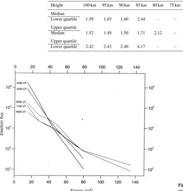
[image:5.595.48.416.217.601.2]Energy, keV
Fig. 5. Spectra deduced from the median electron-density profiles from night to morning.
4 Prediction model for the whole year
The overall results are summarized in Fig. 4, which gives the hourly medians for each height. Note that at 75 km and below the medians were all below the radar threshold. At 80 km the values were above the threshold only between 03:00 and 11:00 UT. Systematic trends are apparant. At 100 and 95 km the ratioNe/Adecreases steadily from the midnight sector
into the daytime, whereas the lower heights show an increase followed by a decrease during the morning hours. The dips at 20:00 UT are probably statistical.
quar-(a)
Solar zenith angle
(b)
[image:6.595.50.288.67.500.2]Solar zenith angle
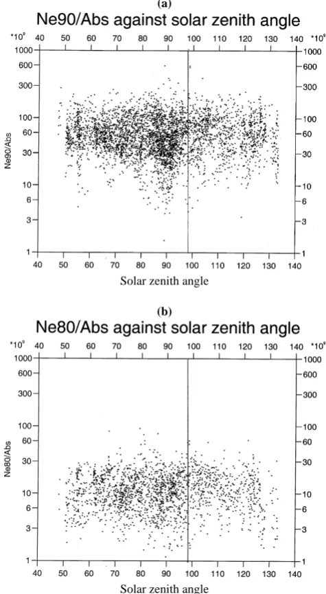
Fig. 6.Ne/Aagainst the solar zenith angle.
tile)/median and median/(lower quartile) are both about 1.5 or 1.6. This means that there is a 50% chance that a single estimate will be within 1.6 of the true value. The spread is somewhat worse at the lower heights.
5 Significance of the diurnal variation
The electron-density profile may be inverted to give an indi-cation of the spectrum of incoming particles that produced it (Hargreaves and Devlin, 1990). Some assumptions have to be made about the atmospheric composition and about the effective recombination coefficient as a function of altitude. Although the absolute values may be questioned, this ap-proach is useful for interpreting changes of profile in terms of a changing spectrum. Treating in this way the median
profiles for 23:00–24:00 UT and each 3 h to 11:00–12:00 UT (Fig. 5) shows a hardening of the typical spectrum with time. The earliest spectrum is almost exponential with characteris-tic energy 6.5 keV, a value consistent with other determina-tions for that time of day (Devlin et al., 1986). Later in the morning, the characteristic energy is considerably greater, about 16 keV. This hardening is also consistent with previ-ous observations of individual events (Hargreaves and De-vlin, 1990).
6 The question of photodetachment
In polar-cap absorption events (PCA), which result from the incidence of solar protons, the level of absorption changes drastically between day and night, according to whether or not the ionosphere is sunlit (Bailey, 1957). Such a transition is expected because the effective electron recombination in the lower ionosphere increases drastically in the absence of daylight, due to attachment of electrons to neutrals and the enhanced formation of cluster ions. PCA occurs lower in the atmosphere than auroral absorption (AA), and attempts to identify the same effect in AA (most notably the analysis by Armstrong et al., 1977) have failed to find one.
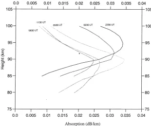
In Fig. 6 we show the quantity Ne/A against the solar
zenith angle (χ), for two altitudes. It will be noted that there is no sharp change betweenχ = 90 and 100◦, as would be the case in PCA. We note, further, that the absorption pro-files (Fig. 7) corresponding to the spectra of Fig. 5 peak be-tween 90 and 95 km; the contribution at and below 75 km is likely to be small. Incoherent-scatter radar studies of PCA, however, show that most of the day/night variation of elec-tron density in those events is selec-trongly height dependent, and is rather small above 75 km (Reagan and Watt, 1976; Col-lis and Rietveld, 1990; Hargreaves et al., 1993). For large ionisation rates, such as those considered in the present con-text (absorption larger than 0.5 dB), the cluster ledge is most likely to be always below 80 km. We conclude that the diur-nal variation shown in Fig. 4 and Table 1 is a consequence of a changing electron spectrum, not of solar illumination.
7 Seasonal variation
The scheme described above takes into account daily but not seasonal variations. To include both variables requires the data to be sorted into 288 boxes to cover each hour of each month, and since the distribution is uneven some of these boxes will contain too few data points for a significant result. Therefore, median values of the ratio Ne/A were derived
Absorption (dB/km)
Fig. 7. Partial absorption profiles corresponding to the median electron-density profiles in the night-to-morning sector.
than 10% should not be considered significant. Differences of more than 50% are likely to be significant.
The best coverage across all months is between 04:00 and 07:00 UT. We can also compare the variations during the day by taking together November to March (as winter) and July to August (as summer), though both these groups lack data from 14:00 to 20:00 UT. The reader may like to draw his or her own conclusions, but the authors offer the following com-ments:
1. At 100 and 95 km, the value of electron density corre-sponding to 1 dB absorption is relatively high in sum-mer around 00:00 UT, but relatively low for several hours before that.
2. At 90 km, the summer maximum at 00:00 UT has van-ished, though values are still low before that time. 3. At 85 km, the low values before 00:00 UT are now
be-low the threshold. There is now also a dip during the early morning (05:00 to 07:00 UT).
4. At 80 km, all summer values are low relative to those at other times of the year.
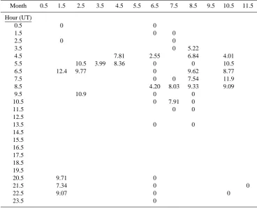
For a given spectrum of incoming energetic electrons, the ionization rate and the effective recombination coefficient, and, therefore, the ionization profile, are all influenced by the vertical profiles of density and pressure in the meso-sphere. Further, the resulting radio absorption depends on the electron-neutral collision frequency, which is also pressure dependent. Direct measurements of atmospheric density at high latitude show a reduction in summer at 100 and 95 km,
and a summer increase at 85 and 80 km. The seasonal vari-ations indicated by Tables A1–5 may well be a consequence of mesospheric changes, but due to the inherent limitations of the data they should be regarded as indications rather than definitive determinations.
8 Conclusions and discussion
1. An analysis of incoherent-scatter and riometer data over a period of 8 years, including more than 4000 individ-ual measurements, shows that an observation of auroral radio absorption may be interpreted to estimate the ap-proximate electron density at heights between 100 and 80 km. The results presented apply only if the absorp-tion is at least 0.5 dB. The results are given in terms of the medians, and upper and lower quartiles of the electron density, corresponding to 1 dB absorption mea-sured with a 27.6 MHz riometer pointed vertically. 2. The uncertainty of the procedure is such that at the
greater heights (100, 95 and 90 km) the estimate will be accurate to within a factor of 1.6 on 50% of the oc-casions. At lower heights the error appears to be rather worse.
quartile could be specified at 80 and 75 km, but not at 70 km.
4. Since the typical spectrum of incoming energetic trons varies with the time of day, the estimates of elec-tron density show a diurnal variation. There is no evi-dence that solar illumination has any effect at 80 km or above.
5. Dividing the data according to both time-of-day and season suggests that a seasonal effect is also present, but due to data limitations the actual values should be treated with caution.
The absorption values used in this investigation are those actually measured by a simple riometer system using a ver-tical 5-element Yagi antenna. It is estimated that such an antenna records absorption about 20% greater than would be measured by an ideal system having a zenithal pencil beam. This factor should be taken into account where appropriate. Acknowledgements. We thank P. Stauning for providing the riome-ter data and M. Harrich for the original data processing. EIS-CAT is supported by Finland (SA), France (CNRS), Germany (MPG), Japan (NIPR), Norway (NFR), Sweden (NFR) and the UK (PPARC).
Topical Editor M. Lester thanks C. Hall and another referee for their help in evaluating this paper.
References
Armstrong, R. J., Berkey, F. T., and Melbye, T.: The day to night absorption ratio in auroral zone riometer measurements, Planet. Space Sci. 25, 1193–1198, 1977.
Bailey, D. K.: Disturbances in the lower ionosphere observed at VHF following the solar flare of 23 February 1956 with particular reference to auroral-zone absorption, J. Geophys. Res., 62, 431, 1957.
Collis, P. N. and Rietveld, M. T.: Mesospheric observations with the EISCAT UHF radar during polar cap absorption events: 1. Electron densities and negative ions, Ann. Geophysicae, 8, 809, 1990.
Devlin, T., Hargreaves, J. K., and Collis, P. N.: EISCAT observa-tions of the ionospheric D region during auroral radio absorption events, J. Atmos. Terr. Phys., 48, 795, 1986.
Friedrich, M. and Kirkwood, S.: The D-region background at high
latitudes, Adv. Space Res., 25, 15, 2000.
Friedrich, M., Harrich, M., Torkar, K. M., and Stauning, P.: Quanti-tative measurements with wide-beam riometers, J. Atmos. Solar-Terr. Phys., 64, 359, 2002.
Hargreaves, J. K. and Cowley, F. C.: Studies of auroral radio absorp-tion events at three magnetic latitudes I. Occurrence and statisti-cal properties of the events, Planet. Space Sci., 15, 1571, 1967. Hargreaves, J. K.: Auroral absorption of HF radio waves in the
ionosphere – a review of results from the first decade of riome-tery, Proc. IEEE, 57, 1348, 1969.
Hargreaves, J. K. and Devlin, T.: Morning sector electron precipita-tion events observed by incoherent scatter radar, J. Atmos. Terr. Phys., 52, 193, 1990.
Hargreaves, J. K., Shirochkov, A. V., and Farmer, A. D.: The po-lar cap absorption event of 19–21 March 1990: recombination coefficients, the twilight transition and the midday recovery, J. Atmos. Terr. Phys., 55, 857, 1993.
Hunsucker, R. D.: Simultaneous riometer and incoherent scatter radar observations of the auroral D-region, Radio Science, 9, 335, 1974.
Jacobsen, T. A. and Friedrich, M.: Electron density measurements in the lower D-region, J. Atmos. Terr. Phys., 41, 1195, 1979. Mechtly, E. A.: Accuracy of rocket measurements of lower
iono-sphere electron density concentrations, Radio Science, 9, 373, 1974.
Ranta, A., Ranta, H., Turunen, T., Silen, J., and Stauning, P.: High resolution observations of D-region by EISCAT and their com-parison to riometer measurements, Planet. Space Sci., 33, 583, 1985.
Reagan, J. B. and Watt, T. M.: Simultaneous satellite and radar studies of the D-region ionosphere during the intense solar parti-cle events of August 1972, J. Geophys. Res., 81, 4579, 1976. Rees, M. H.: Auroral ionization and excitation by incident energetic
electrons, Planet. Space Sci., 11, 1209, 1963.
Appendix
Table A1. Median Electron density at 100 km for 1 dB absorption
Month 0.5 1.5 2.5 3.5 4.5 5.5 6.5 7.5 8.5 9.5 10.5 11.5
Hour (UT)
0.5 180 341
1.5 189 144
2.5 182 140
3.5 78.6 178
4.5 155 143 142 166
5.5 128 66.5 88.7 103 109 128
6.5 58.9 104 118 103 115
7.5 111 62.5 76.3 81.2
8.5 101 46.6 75.3 52.0
9.5 54.6 97.8 91.4
10.5 114 76.6 70.5
11.5 111 76.6
12.5
13.5 95.7 56.9
14.5 15.5 16.5 17.5 18.5 19.5
20.5 287 64.0
21.5 200 84.6 102
22.5 208 103 244
23.5 280
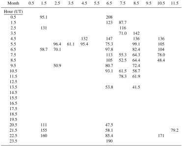
Table A2. Median Electron density at 95 km for 1 dB absorption
Month 0.5 1.5 2.5 3.5 4.5 5.5 6.5 7.5 8.5 9.5 10.5 11.5
Hour (UT)
0.5 95.1 208
1.5 123 87.7
2.5 131 116
3.5 71.0 142
4.5 132 147 136 136
5.5 96.4 61.1 95.4 75.3 99.1 105
6.5 58.7 70.1 97.8 82.4 104
7.5 113 55.3 64.3 78.0
8.5 105 52.5 64.4 48.4
9.5 50.9 80.7 72.4
10.5 93.1 61.5 58.7
11.5 78.3 61.9
12.5
13.5 53.8 41.5
14.5 15.5 16.5 17.5 18.5 19.5
20.5 111 47.5
21.5 155 58.1 79.2
22.5 160 85.4 171
[image:9.595.111.483.436.733.2]Table A3. Median Electron density at 90 km for 1 dB absorption
Month 0.5 1.5 2.5 3.5 4.5 5.5 6.5 7.5 8.5 9.5 10.5 11.5
Hour (UT)
0.5 40.6 41.1
1.5 44.4 39.2
2.5 61.7 72.5
3.5 51.4 85.5
4.5 78.4 108 82.1 57.6
5.5 48.3 41.2 84.8 42.0 71.5 79.9
6.5 53.7 58.8 61.4 74.7 71.0
7.5 78.6 61.2 60.3 56.9
8.5 68.2 63.3 52.3 37.9
9.5 48.4 49.2 48.6
10.5 53.4 57.7 50.0
11.5 57.9 51.4
12.5
13.5 30.9 32.8
14.5 15.5 16.5 17.5 18.5 19.5
20.5 49.5 21.1
21.5 87.6 30.7 34.0
22.5 86.4 39.2 70.3
23.5 46.9
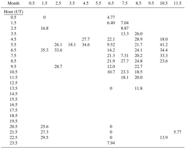
Table A4. Median Electron density at 85 km for 1 dB absorption
Month 0.5 1.5 2.5 3.5 4.5 5.5 6.5 7.5 8.5 9.5 10.5 11.5
Hour (UT)
0.5 0 4.77
1.5 6.40 7.04
2.5 16.8 8.87
3.5 13.3 26.0
4.5 27.7 22.1 28.9 18.0
5.5 26.1 18.1 34.6 9.52 21.7 41.2
6.5 35.3 33.6 14.2 24.1 34.4
7.5 21.3 7.31 20.2 33.3
8.5 21.9 27.7 24.8 23.6
9.5 28.7 12.0 22.7
10.5 10.7 23.3 18.5
11.5 18.1 20.0
12.5
13.5 0 11.8
14.5 15.5 16.5 17.5 18.5 19.5
20.5 25.6 0
21.5 27.3 0 5.77
22.5 29.5 0 13.9
[image:10.595.111.483.436.733.2]Table A5. Median Electron density at 80 km for 1 dB absorption
Month 0.5 1.5 2.5 3.5 4.5 5.5 6.5 7.5 8.5 9.5 10.5 11.5
Hour (UT)
0.5 0 0
1.5 0 0
2.5 0 0
3.5 0 5.22
4.5 7.81 2.55 6.84 4.01
5.5 10.5 3.99 8.36 0 0 10.5
6.5 12.4 9.77 0 9.62 8.77
7.5 0 0 7.54 11.9
8.5 4.20 8.03 9.33 9.09
9.5 10.9 0 0
10.5 0 7.91 0
11.5 0 0
12.5
13.5 0 0
14.5 15.5 16.5 17.5 18.5 19.5
20.5 9.71 0
21.5 7.34 0 0
22.5 9.07 0 0