Measuring Light and Geometry Data of Roadway Environments with a Camera

Measuring Light and Geometry Data of Roadway

Environments with a Camera

Hongyi Cai*, Linjie Li

Department of Civil, Environmental & Architectural Engineering, The University of Kansas, Lawrence, USA Email: *[email protected]

Received September 23, 2013; revised October 27; 2013; accepted November 21, 2013

Copyright © 2014 Hongyi Cai, Linjie Li. This is an open access article distributed under the Creative Commons Attribution License, which permits unrestricted use, distribution, and reproduction in any medium, provided the original work is properly cited. In accor-dance of the Creative Commons Attribution License all Copyrights © 2014 are reserved for SCIRP and the owner of the intellectual property Hongyi Cai, Linjie Li. All Copyright © 2014 are guarded by law and by SCIRP as a guardian.

ABSTRACT

Evaluation of the conspicuity of roadway environments for their environmental impact on driving performance is vital for roadway safety. Existing meters and tools for roadway measurements cannot record light and geome-try data simultaneously in a high resolution. This study introduced a new method that adopted recently devel-oped high dynamic range (HDR) photogrammetry to measure the luminance and XYZ coordinates of millions of points across a road scene with the same device—a camera, and a MatLab code for data treatment and visualization. To validate this method, the roadway environments of a straight and flat section of Jayhawk Boulevard (482.8 m long) at Lawrence, KS and a roundabout (15.3 m in diameter) at its end were measured under clear and cloudy sky in the daytime and at nighttime with dry and wet pavements. Eight HDR images of the roadway environments under different viewing conditions were generated using the HDR photogrammetric techniques and calibrated. From each HDR image, synchronous light and geometry data were extracted in Radiance and further analyzed to identify

po-tential roadway environmental hazards using the MatLab code

HDR photogrammetric measurement with current equipment had a margin of errors for geometry measurement that varied with the measuring distance, averagely 23.1% - 27.5% for the Jayhawk Boulevard and 9.3% - 16.2% for the roundabout. The accuracy of luminance measurement was proven in the literature as averagely 1.5% - 10.1%. The camera-aided measurement is fast, non-contact, non-destructive, and off the road, thus, it is deemed more efficient and safer than conventional ways using meters and tools. The HDR photogrammetric techniques with current equipment still need improvements on accuracy and speed of the data treatment.

KEYWORDS

Measurement; Geometry; Light; Roadway Environment; High Dynamic Range Photogrammetry

1. Introduction

The conspicuity of roadway environments is affected by many factors, including the transitory lighting and weather conditions, the geometry and layout of roadway elements, the legibility of roadway signs and plaques, and the visibility of traffic control signals, pavement markings and markers, object markers, delineators, channelizing devices, and pedestrian hybrid beacons, etc. As a result, the conspicuity of roadway environments varies over time under different viewing conditions, e.g., in the daytime or at nighttime; in sunny, rainy, foggy, or snowy weathers; with dry or wet pavements, etc.

When the conspicuity of essential roadway environ-ments (e.g., intersections) is harmed at nighttime or even in the daytime under less-than-optimal viewing condi-tions, roadway lighting is often needed to increase the visibility of the pavement, traffic control devices, and on-road/off-road hazards to facilitate drivers conducting driving tasks safely. However, roadway lighting with low quality may provide insufficient light, cast shadows on the road pavement, or bring discomfort glare to motorists and pedestrians, which all reduce the visibility of the roadway environments.

Therefore, evaluation of the roadway environments is vital for their environmental impact on driving perfor-mance and roadway safety. Routine measurements of the *

45

roadway environments could help to maintain a good conspicuity of essential roadway elements, and also iden-tify potential roadway hazards (e.g., illegible roadway signs, insufficient light on pavement, glaring roadway lighting, etc.) that may jeopardize the roadway’s visibili-ty and the drivers’ visual comfort. Both light and geome-try data of the roadway environments need to be meas-ured simultaneously.

What light and geometry data need to be measured in the roadway environments? Lighting metrics measured on the road often include surface illuminance and lu-minance, their spatial variations, luminance contrast be-tween a target and its background, etc. The commonly measured geometries of the roadway environments in-clude size and shape of the pavement, sidewalks, road-way markings and markers, and surrounding objects and their distances, etc. In addition, the acquired light and geometry data, if concurrent, are used for derivation of some advanced metrics for timely roadway environment assessment. Such metrics with which the light and geo-metry data are jointly involved include visibility of ob-jects on the road, legibility of roadway signs, discomfort glare of roadway lights, roadway surface reflectance, uniformity of pavement light distribution, and luminance gradient (the frequency of the spatial luminance variation) [1] across the roadway environment, etc.

How to measure light and geometry data in the road-way environments? Conventionally, meters and tools have been used. Minolta LS-100 luminance meter, Mi-nolta T-10 lux meter, and MiMi-nolta CL-200A chroma me-ter are popular handheld light meme-ters. Handheld retroref-lectometers, such as Delta LTL-X, Mirolux Ultra 30, can provide traceable, accurate, repeatable and reproducible retroreflectivity measurements. For measuring distances and angles, rulers, tapes, wheel rolls, laser distance me-ters, laser rangefinders, protractors, and magnetic angle locators have been used. The measurement using meters and tools is a reliable but tedious point-by-point process with very low measurement resolution (number of meas-ured points per surface area). The dynamic daylight, transient weather, moving traffic, and other changing viewing conditions on road all affect the accuracy of overall roadway measurement using meters and tools that take hours or even longer [2,3]. In addition, it is danger-ous for workers to conduct the measurement on road with active traffic flow.

To solve these problems, remote sensing technologies are preferred for fast, non-contact, non-destructive and off-road measurement. This paper introduced a new camera-aided method for measuring millions of syn-chronous light and geometry data of the roadway ronments. To validate this method, the roadway envi-ronments on Jayhawk Boulevard in Lawrence, KS and a roundabout at its end were measured under clear and

cloudy sky in the daytime and also at nighttime with dry and wet pavements.

2. Literature Review

In the past 20 years, several non-contact measurement techniques were developed for measuring the roadway geometry or light. They are reviewed below.

2.1. Roadway Geometry Measurement

Drakopoulos and Ornek developed a non-contact method for measuring roadway geometry [4]. A vehicle was used to carry a distance-measuring device, a vertical gyros-cope, and a gyrocompass. Data collected include odome-ter reading, gradient, transverse slope, and compass reading. From these data, an algorithm was developed for calculating the roadway geometry, including road length, deflection angle, and degree of curves. The conventional inertial data logging and advanced GPS (global position-ing system) data loggposition-ing were used in their study, both had low accuracy. Inertial hardware has acceleration ef-fect on readings, which needs frequent calibration. Al-though the GPS technology has no acceleration effect, atmospheric disturbances, receiver errors and other fac-tors reduce the accuracy of GPS devices. Due to these problems, the measurement errors of this algorithm were relatively large, up to 63.8%.

GPS was also used for measuring roadway geometry. Nehate and Rys used GPS data to calculate stopping- sight distance of highways [12]. A profiling van collected GPS raw data such as latitude, longitude, and altitude of road surface and sight obstructions, which were trans-formed into B-spine curves. Drivers’ sight line inter-sected with these two curves. By examining the intersec-tions, the sight distance was derived. The measurement error was ±0.2 m. This algorithm was not capable of showing the actual image of sight obstructions and de-tailed information of the road surface. Castro et al. used a Leica System 500 GPS to track the geometry of highway system [13]. The GPS were mounted on a vehicle to measure the coordinates when the vehicle was moving along the highway, with maximum error of 1 m. Koc also used GPS for rail-track surveying [14]. He used a trailer equipped with GPS antennas. The GPS measured the coordinates of the trailer at a frequency of 20 Hz with error of 0.01 - 0.03 m. It was assumed that the rail-track was on a horizontal plane, thus, lacked information for 3D modeling. This method was also not capable of showing detailed visual information of the scene.

Tsai and Li used a laser system to detect the cracks on the pavement [15]. Two laser units were mounted on a vehicle to cover a full lane width. Laser beams were pro-jected on the pavement. CMOS cameras were used to detect the reflected light of the laser. Likewise, Amarasiri

et al. used a CCD camera for measuring pavement

ma-cro-texture and wear of pavement [16,17]. The CCD camera sensed the optical reflection properties of the pavement and recorded them on the image.

2.2. Roadway Light Measurement

Arditi et al. developed a system called LUMINA [18]. This system deployed an analog video camera and a photometer to record the image and luminance value of the safety vests synchronously. A device called AI-GOTCHA was used to convert the frames of the analog videotape to BMP format. The luminance values of the vests were calculated using RGB values extracted from the image. The luminance values were also measured with a photometer for physical calibration of the calcu-lated luminance. This study had two limitations. First, the analog/digital conversion introduced new errors. Second, the camera had a very low resolution of only 400 lines, which was inadequate and outdated compared to digital cameras.

To improve, other researchers used digital cameras for recording the roadway luminance. Zatari et al. used two CCD cameras mounted on top of a vehicle for measure-ment of glare, luminance and illuminance of road light-ing [19]. Due to the limited field of view of the cameras, one camera was aiming straight forward to cover the road,

the other was aiming upward to photograph the lumi-naires on poles. The measurement error of absolute illu-minance was within 15 lx, while the average error of luminance measurement was 0.3185 cd/m2. Likewise, Aktan et al. used a CCD photometer that was mounted outside a vehicle and automatically took photos of the road scene while the vehicle was moving [20]. The reso-lution of the CCD photometer was 1 megapixel and the measurement error of road luminance was within 10%. Ekrias et al. developed a technique to measure the lu-minance on road with a ProMetric 1400 photometer [2,3]. The CCD camera of the photometer captured the scene and luminance values a across the whole scene in a few seconds. Due to the reduced measurement time, the error of this CCD photometer system was reduced to ±3%. However, the pixel resolution of this CCD ProMetric 1400 photometer is only 500 × 500, which was not enough to measure large scenes. Armas and Laugis used an LMK camera developed by the TechnoTeam Compa-ny for measuring roadway luminance [21,22]. The LMK camera could record both the image and luminance val-ues of the scene with a pixel resolution of 5184 × 3456 for image acquisition and 2592 × 1728 for luminance mapping [23]. Ylinen et al. also used the LMK Mobile Advanced luminance measuring camera for evaluation of LED street lighting [24]. In spite of their potentials for wide uses in roadway environments, all these measure-ment techniques proposed by Ekrias et al. [2,3], Aktan et al. [20], Armas and Laugis [21,22], and Ylinen et al. [24] required high-cost equipment.

47

2.3. Roadway Geometry and Light Measurement

Other researchers developed techniques to measure both geometry and light of the roadway environments. Zhou et al. mounted a light meter and a longitudinal distance measurement instrument on a vehicle [28]. A computer was used to control these devices for measuring the loca-tion and illuminance of the road elements while the ve-hicle was moving. This technique did not use the same device to measure the concurrent light and geometry data. As a result, the light and geometry data obtained sepa-rately were not aligned at the same measurement points. It also had low measurement resolution, a problem affi-liated with the conventional meters.

Gutierrez et al. developed a camera-aided method to measure the luminance of a traffic sign lighted by the vehicle headlights solely from the driver’s view, as well as its distance [29]. A van was equipped with two mo-nochrome CCD cameras mounted close to the driver, and LEDs in the front to simulate the headlight. When the van was moving, a computer was used to switch the LEDs on and off. One camera took an image with the LEDs turned on, later the other camera took an image with the LEDs turned off. From the two consecutive im-ages, luminance values of the traffic sign were extracted. The difference between the extracted luminance values of the two images was assumed the luminance of the traffic sign lighted by the LEDs only. This technique could exclude the influence of ambient light from road lamps and the headlamps of other vehicles. The distance from the van to the sign was calculated from the norma-lized size of the sign and the traveled distance of the van over the time delay when the two consecutive images were photographed. Nonetheless, Gutierrez et al.’s tech-nique had two insufficiencies. First, their techtech-nique did not capture a high dynamic range of light in the roadway environment, since both cameras, which lacked a superb image sensor, did not photograph the scene via sequential exposures. Second, an accurate measurement of lumin-ance is dependent on the measurement direction. The luminance differential extracted from the two consecu-tively photographed images was not truly the sign lu-minance when lighted only by the LEDs, because the viewing direction from the cameras to the sign was changed over the time delay.

3. Research Gap and Problems

The non-contact measurement techniques developed by those researchers aforementioned are of great improve-ment upon meters and tools in light of the measureimprove-ment speed, resolution, overall accuracy under varying road-way conditions (due to the shortened measurement time), and the capability of measuring large non-uniform

sur-faces. However, none of those techniques is able to measure geometry and light level of the entire roadway environment simultaneously with the same device. The separated measurements increase the field measurement labor, slow the data collection, and cause difficulties in follow-up data alignment. Capturing synchronous light and geometry data across a roadway environment with the same device can speed up the measurement in that there is no need to measure twice, and no pixels on the photographic images are wasted in data treatment later (e.g., in the study by Wu and Tsai [7]. The concurrent light and geometry data could serve more needs than separately measured data for roadway environment as-sessment, e.g., visibility of objects on the road, legibility of roadway signs, glare, uniformity, roadway surface reflectance, and luminance gradient, etc.

On the other hand, on-road measurement, using either handheld meters and tools or non-contact measurement equipment mounted on vehicles running on road, is harmful for roadway safety and overall efficiency. Dur-ing the measurement, the workers and instrumented ve-hicles constantly on the road could hinder the roadway traffic, and increase the risk of rear-end collisions. Off- road non-contract measurement does not interrupt road-way traffic, thus, is safer. The HDR photography could be used for luminance mapping an entire roadway envi-ronment off the road by approximating the sightline and field of view of a typical observer. It has the attraction due to its low entry barrier, extraordinarily high resolu-tion, rapid measurement speed, and acceptable accuracy. Yet the HDR photography does not record any geometry of the roadway scene. The geometric features, which are needed for roadway condition evaluation, have to be measured separately.

Recently, based on the HDR photography, Cai devel-oped the HDR photogrammetry for measurement of synchronous light and geometry data of an entire scene with the same device (the camera) [30]. When used for close- and middle-range scenes (i.e., ≤8.14 m), the

4. The HDR Photogrammetric Measurement

of Roadway Environments

The HDR photogrammetry was developed for acquisition of luminance of millions of target points across a scene and their right-handed Cartesian coordinates XYZ in the field [30]. It deploys a consumer grade digital camera fitted with a standard, wide-angle, or fisheye lens mounted on a portable photogrammetric measurement platform. The camera is mounted in the test scene with yaw angle κ, pitch angle η, and roll angle φ related to the world coordinates XYZ, following the right hand rule. A notebook computer controls the camera to take multiple LDR photographs of the test scene, which are later fused into an HDR image. The HDR image plane is located on the image sensor of the camera, with pixel coordinates xz. Any single target plane, on which the target points are randomly distributed, also has yaw angle θ, pitch angle τ, and roll angle ρ in light of the world coordinates XYZ. A target P (X, Y, Z) and a reference point Pi (Xi, Yi, Zi) are both located on the target plane. The position (Xi, Yi, Zi) of the reference point Pi is measured in the field. Mini-mum three, ideally four, reference points are needed for identifying a target plane. If the yaw, pitch, and roll an-gles of the target plane, e.g., a flat road pavement, are known, then only one reference point is needed. Aided by the reference point Pi, the location (X, Y, Z) of the target P in the field can be converted from its pixel loca-tion (x, z) on the HDR image, by using some photo-grammetric transforming equations [30]. Meanwhile, the luminance value of the target P can be obtained from the HDR image. Then it is possible to extract the luminance values and XYZ coordinates of the entire scene from the HDR image at pixel level.

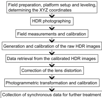
Below is an introduction to the deployment of the HDR photogrammetry for roadway measurement, in-cluding the field measurement procedure and data treat-ment. Figure 1 is the flow chart to depict the field mea-surement procedure and follow up data treatment.

4.1. Field Measurement Procedure

Below is a protocol divided into five steps of the HDR photogrammetric measurement in the field.

Step 1: field preparation. The camera location in the road scene may be any typical viewpoint of the observer (e.g., a driver, a pedestrian, etc.). An off-road mounting location is preferred for the benefit of roadway safety and traffic flow, if the sightline of the observer could be ap-proximated off the road. With the right lens, the camera’s field of view shall cover all interested target points in the roadway environments. In addition, four reference points need to be identified for each target plane (e.g., pavement, sidewalk, roadway sign, etc.). Common reference points include visible roadway marks, edges of the curb, or field

Figure 1. The flow chart of the field measurement and fol-low up data treatment.

objects such as light poles, plants, etc. Some reference objects, such as wood white boards, could be placed on interested points for the benefit of meter measurement. An X-Rite 18% gray checker is also mounted on a tripod and placed close to the camera shooting line for photo-metric calibration.

Step 2: platform setup and leveling. The camera is then mounted on a 3D angular measurement tripod head [30], which is mounted on a heavy-duty flat head tripod and leveled. The tripod head has an adjustable base with three screws for micro-adjustment to ensure the platform is truly horizontal at its initial position. The tripod head has three angular dials on the base, the front and the side, respectively, to record the aiming yaw, pitch and roll angles of the camera with a precision of 0.1˚. A Dell La-titude notebook computer is used for remote control of the camera and data recording.

Step 3: determining the XYZ coordinates. In roadway scenes, the World Coordinate System (WCS) is used, which has fixed coordinates—X (east), Y (north), Z (up). The origin point O (0, 0, 0) of the photogrammetric coordinates is overlapped at the optical center of the camera. To determine the initial yaw pitch and roll an-gles (κXYZ, ηXYZ, φXYZ) of the XYZ coordinates, a compass is put on the platform to adjust the 3D angular measure-ment tripod head until the camera is aiming north. Yaw angle κXYZ and pitch angle ηXYZ are recorded from the angular dials. Roll angle φXYZ is assumed 0˚ for roadway measurement.

Step 4: HDR photographing. The camera is manually

illumin-49

ance at the lens is used to control the light measurement in the field and as an input of potential glare calculation (not covered in this study). The Dell notebook computer is used to remotely control the camera to take a total of 18 LDR photographs via sequential exposures (1/4000 s to 30 s @ aperture of f/5.0). Some of them fallen in a good exposure range are fused into a raw HDR image. During the photographing, the luminance meter Minolta LS-100 mounted beside the camera is used to measure the luminance of the X-Rite 18% gray checker for pho-tometric calibrations of the raw HDR image.

Step 5: field measurements and calibration. From the three dials of the tripod head, the camera’s initial aiming direction (κ0, η0, φ0) is recorded. The actual aiming an-gles (κ, η, φ) are calculated as κ = κ0− κXYZ, η = η0−

ηXYZ, φ = φ0−φXYZ. Next, the camera is dismounted from the tripod head and replaced with a laser distance meter Leica DISTO™ D5 for measuring the distance di of the reference point Pi. If faraway points exceed the mea-surement range (650 ft) of the laser distance meter, a Bushnell EliteTM 1600 laser rangefinder is used to replace the laser distance meter. The aiming angles of Pi (ϕi,a, αi,a) are then recorded from the angular dials on the side and base of the tripod head. Note that due to different optical structures, when replacing the camera with the laser dis-tance meter or the rangefinder, the aiming direction may change. To calibrate this error, the laser distance meter or the rangefinder is re-aimed to the same aiming point of the camera. The new aiming direction (κm0, ηm0, φm0) is recorded from the three angular dials. The offsets of the aiming angles are calculated using Equation (1). The off-axis angles are then calculated using Equation (2). The four reference points Pi (Xi, Yi, Zi) (i = 1, 2, 3, 4) are later calculated using Equation (3).

0 0

0 0 m m κ κ κ η η η

∆ = −



∆ = −

 (1)

,

, i i a XYZ

i i a XYZ

φ φ κ κ

α α η η

= − − ∆ 

 = − − ∆

 (2)

( )

( )

cos sin

cos cos

sin

i i i

i

i i i i

i i i

d X Y d Z d α φ α φ α  −    _{ }  _{ = − }      _{  }  _{  } (3)

4.2. Data Treatment

The field-measured data are then treated using personal computers at six steps below, which are numbered after the previous five steps.

Step 6: generation of raw HDR images. Raw HDR images are generated from an appropriate exposure range of those LDR photographs using Photosphere or Ra-diance [26]. Before that, if necessary, the LDR

photo-graphs need treatments to filter any unwanted voltage bias, dark current and conductive noise, and fixed pattern noise [26,31].

Step 7: calibrations of the raw HDR images. The raw

HDR images are then calibrated in Radiance, including, in order, 1) vignetting effect correction, which corrects the light drop-off in the periphery of the field of view, and 2) photometric calibration, which corrects the lu-minance differential between the camera-aided mea-surement and the luminance meter meamea-surement of the X-Rite 18% gray checker [26].

Step 8: data retrieval from the calibrated HDR images.

Of every single pixel, the luminance and pixel location

Ppix (xpix, zpix) are extracted from the calibrated HDR im-ages in Radiance, using the command “pvalue” (pvalue -o -h -b $HDR > L_$HDR.txt). The output text file en-closes per-pixel luminance values across the scene in a data format of {xpix, zpix, luminance}. In addition, from the pixel location, the distorted geometric coordinate Pd (xd, zd) of the target point P on the image plane xz is then derived [30].

Step 9: correction of the lens distortion. A wide-angle lens often has radial distortions that need corrections for geometry measurement. Of every single pixel, the dis-torted geometric coordinates Pd (xd, zd) are then corrected as undistorted Pu (xu, zu). More details of the correction models are available in the literature [30].

Step 10: photogrammetric transformation & calibra-tion. The XYZ coordinates of the target point P in the field are then transformed from its undistorted geometric coordinates Pu (xu, zu) on the image plane, using some transformation equations developed by Cai [30]. The local coordinates X′Y′Z′ of the target point P are first calculated from Pu (xu, zu). Then the local X′Y′Z′ coord i-nates are converted back to the WCS coordii-nates P (X, Y, Z) with the aid of the field measured XYZ coordinates of the reference points. The last step is the photogrammetric calibration using the four reference points. The average geometric deviation between their measured and the cal-culated XYZ coordinates is used to further calibrate the P (X, Y, Z) [30].

gradient direction} [1]. The underlined coordinate of each map is in pseudo color. The MatLab code for such data treatment and image plotting is available online

5. Validation of the Method in the Field

5.1. Field Measurements

The HDR photogrammetric measurement is fast, non- contact, non-destructive, and off the road. To validate this method, the roadway environments of a straight and flat section of Jayhawk Boulevard (482.8 m long) at Lawrence, KS and a roundabout (15.3 m in diameter) at its end were measured. The Jayhawk Boulevard went through the campus of the University of Kansas. On both sides of this road, there were buildings, trees, light poles, traffic signs, statues, newspaper booth, etc. The rounda-bout had three asymmetrical non-straight approaches.

In this study, the Canon camera EOS rebel T2i with an 18-mega pixel CMOS sensor fitted with a Sigma EX DC HSM 10 mm diagonal fisheye lens was deployed. The HDR photogrammetric measurement platform is shown

in Figure 2, on which the camera was mounted. The

op-timized lens aperture size of f/5.0 was used based on previous studies [26,31]. Several pieces of wood white boards were placed on interested locations serving as the target and reference points. In both test scenarios, an off-road measuring location was chosen.

For measuring Jayhawk Boulevard, four HDR images were generated under clear or cloudy sky in the daytime, and also at night with dry or wet pavement, as shown in

Figure 3, which were photographed at the same off-road

location aiming at the same direction.

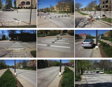
In addition, a total of 24 points on Jayhawk Boulevard were selected for measurement of their XYZ coordinates, as shown in Figure 4. Points 1 - 4 were reference points. Others were target points. Points 5 - 11 and 15 - 20 were the centers of crosswalk strips. Point 14 was the focusing target of the camera, which was a blue newspaper booth. Points 12 and 13 were the bottoms of trees. Points 21 - 23 were the bottoms of light poles. Point 24 was a traffic booth at the end of the road. Independent of various viewing conditions, the field measurement of the 24 points was conducted in the daytime under clear sky due to better legibility of the far targets. White wood boards were placed at those points to help the laser distance me-ter and rangefinder acquire the targets.

The roadway environment at the roundabout was also measured off the road. Figure 5 shows the four HDR images taken under clear or cloudy sky in the daytime, and also at night with dry or wet pavement.

A total of 21 points, as shown in Figure 6, were measured in the field in the daytime under clear sky for their XYZ coordinates. Points 1 - 6 were the top left cor-ners of the crosswalk strips. Points 7 - 13 were white

(a) (b)

Figure 2. The HDR photogrammetric measurement plat-form used (a) on Jayhawk Boulevard, and (b) at the roun-dabout.

(a) (b)

(c) (d)

Figure 3. Four HDR images of Jayhawk Boulevard taken at the same off-road location aiming at the same direction but under different environmental conditions: (a) Daytime, clear sky, (b) Daytime, cloudy sky, (c) Nighttime, dry pave- ment, and (d) Nighttime, wet pavement.

wood boards placed on the curb. Points 7 and 13 were on roadside. Points 8 - 10 were on the central island. Points 11 and 12 were on a deflection island. Points 14 - 16 were the centers of two “STOP” signs. Points 17 - 21 were corners of deflection markings. Since the rounda-bout was not flat, those 21 points were divided into three groups in data treatment based on their Z coordinates. In each group, the target points had very similar Z values. The first group consists of Points 1 - 8, 17 - 19. Among them, Points 1, 6, 7, and 9 were used as reference points for data treatment. Other points were used as target points to validate the photogrammetric measurement. The second group consists of Points 10, 11, 12, and 16. Points 10 - 12 were used as reference points, while Point 16 was used as a target point. The third group consists of Points 13 - 15, 20 and 21. Points 13, 14, 15 and 20 were used as reference points, while Point 21 was used as a target point.

5.2. Results of Geometry Measurement

51

Figure 4. Locations of the 24 points measured on Jayhawk Boulevard in the daytime under clear sky.

(a) (b) (c) (d)

Figure 5. The four HDR images of the roundabout taken at the same location aiming at the same direction but under differ- ent environmental conditions: (a) Daytime, clear sky, (b) Daytime, cloudy sky, (c) Nighttime, dry pavement, and (d) Night- time, wet pavement.

Figure 6. Locations of the 21 points measured at the roundabout in the daytime under clear sky.

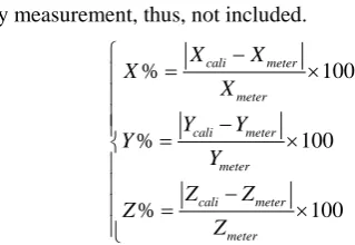
vironments, the calibrated geometric coordinates Xcali,

Ycali, Zcali were calculated from its pixel location extracted from the calibrated HDR image generated in the daytime under clear sky. The calculated Xcali, Ycali, and Zcali were then compared to the coordinates Xmeter, Ymeter, and Zmeter actually measured in the field using the laser distance

geome-try measurement, thus, not included. % 100 % 100 % 100 cali meter meter cali meter meter cali meter meter X X X X Y Y Y Y Z Z Z Z  − = ×    ₋  _{= ×}    ₋  = ×  (4)

Table 1summarizes the measurement errors of the 24

points on Jayhawk Boulevard. Likewise, the geometric errors of measuring the 21 points at the roundabout are shown in Table 2. In Tables 1 and 2, the interquartile range (IQR) covers the most common (the middle 50%) measurement errors in practice (Cai, 2013). It was found that the errors of geometry measurement on Jayhawk Boulevard, regardless of X, Y, or Z coordinate, varied a lot with the measuring distance, e.g., from 5.7% to 39.5% with an interquartile range (IQR) of 14.3% - 37.5% for X coordinate, from 6.8% to 40.3% with an interquartile range (IQR) of 21.1% - 38.6% for Y coordinate, and from 0.6% to 61.6% with an interquartile range (IQR) of 4.4% - 39.4% for Z coordinate. In addition, the average errors of measuring the XYZ coordinates were ranged from 23.1% to 27.5%. The margin of errors for measur-ing the geometry of the roundabout was also very large, 0.1% - 90.0% (X), 0.2% - 52.3% (Y), 0.0% - 137.5% (Z), due to its sloped pavement. The largest error (137.5%) occurred at Z coordinate for approximation of the sloped and curved roundabout pavement. The average errors of the measured XYZ coordinates of the 21 target points were in a range of 9.3% - 16.2% (for XYZ coordinates), with IQR of 1.9% - 16.5% (X), 4.9% - 14.4% (Y), and 0.0% - 2.2% (Z), smaller than those of the longer Jay-hawk Boulevard.

5.3. Results of Light Measurement

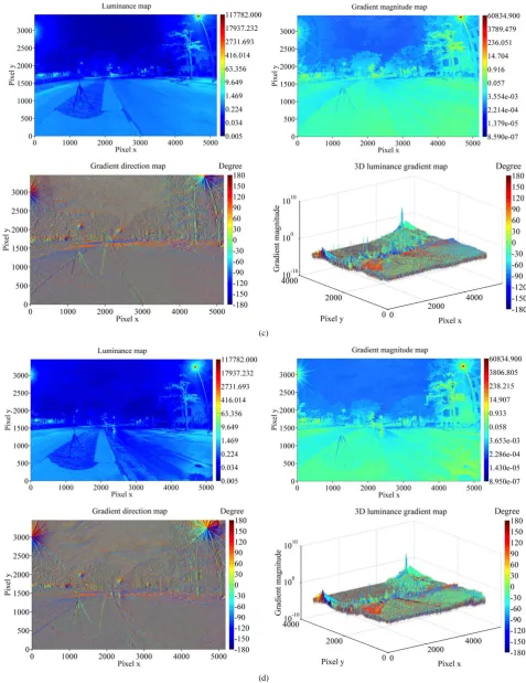
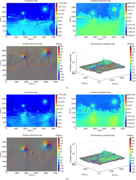
Luminance mapping the two roadway environments was at pixel level. Figures 7and8 show the light distribution maps plotted in MatLab measured on Jayhawk Boulevard and at the roundabout, respectively, in the daytime under clear sky or cloudy sky, or at nighttime with dry or wet pavement. Each map contains 18 millions values. For the benefit of direct comparison, the luminance scale of dif-ferent maps is fixed in a range of 0.00519 cd/m2 (the minimum luminance recorded in those eight HDR im-ages)—117782.0 cd/m2 (the maximum luminance rec-orded). Likewise, the luminance gradient magnitude is set in a fixed range of 8.950 × 10−7 - 60834.900 cd/m2/ pixel. The luminance gradient direction is in a fixed an-gular range of −180˚ - 180˚, measured anticlockwise in light of the x axis of the photographic images (e.g., the angle 0˚ is to the right hand, 90˚ is up, 180˚/−180˚ is to

Table 1. Errors of measuring the XYZ coordinates of the 24 points on Jayhawk Boulevard.

Measurement Errors (%)

X Y Z

Max 39.5 40.3 61.1

Min 5.7 6.8 0.6

Average 25.0 27.5 23.1

Median 24.1 27.1 10.2

IQR 14.3 - 37.5 21.1 - 38.6 4.4 - 39.4

Table 2. Errors of measuring the XYZ coordinates of the 21 points at the roundabout.

Measurement Errors (%)

X Y Z

Max 90.0 52.3 137.5

Min 0.1 0.2 0.0

Average 16.2 12.1 9.3

Median 8.6 8.6 0.0

IQR 1.9 - 16.5 4.9 - 14.4 0.0 - 2.2

the left, −90˚ is down). Figures 7and8 visualize the per- pixel lighting conditions across the two roadway envi-ronments.

The two roadway environments had the highest overall light level in the daytime under clear sky, and the lowest light level at rainy night. At nighttime, the luminance of the wet pavement was lower and less uniform than that of the dry pavement. In particular, puddles that reflected the light of the road lamps to the camera appeared brigh-ter. The overall light distribution in sunny days was less uniform (the gradient magnitude was higher) than that in cloudy days, and than that at night. In particular, the sky on cloudy days was less uniform (the gradient magnitude was higher) than that on sunny days, while the sky un-iformity was the best at night independent of the pave-ment conditions.

53

(a)

(c)

(d)

55

(a)

(c)

(d)

Figure 8. The lighting conditions of the roundabout (a) in the daytime under clear sky, (b) in the daytime under cloudy sky, (c) at nighttime with dry pavement, (d) at nighttime with wet pavement.

57

e.g., buildings, pavement, sidewalks, poles, plants, could still be detected due to changed directions of light reflec-tion on edges.

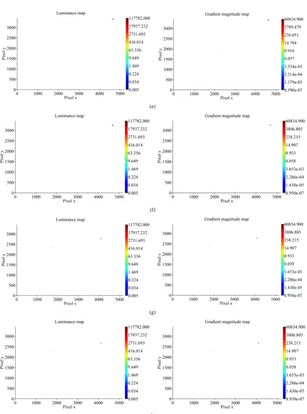
Moreover, those luminance maps and luminance gra-dient magnitude maps shown in Figures 7 and 8 were further treated for identifying potential roadway hazards, including unshielded roadway lamps, too bright pave-ment puddles, extremely high roadway contrasts, and large non-uniform pevement shadows, etc. Any electric light sources brighter than a threshold value of 500 - 700 cd/m2 will cause glare at night [32]. This threshold value could be much higher in the daytime due to increased adaptation level. Extreme light contrasts can also be identified by a threshold luminance gradient magnitude, e.g., 500 - 700 cd/m2/pixel that is consistent with the threshold luminance, whose polarity is shown by the gradient direction. The distracting glare sources and large and sharp pavement shadows will harm the drivers’ de-tection of pavement markings and road targets, thus, need to be identified and eliminated for roadway safety. For demonstration, this study adopted the threshold val-ues of 5000 cd/m2 and 5000 cd/m2/pixel in the daytime and 500 cd/m2 and 500 cd/m2/pixel at nighttime. The number of 5000 was assumed, since the threshold value in the daytime is not a constant which varies with the light adaptation level. The threshold values could be ad-justed for more or less stringent needs. Figure 9 shows the identified potential hazards of the two roadway envi-ronments at their pixel locations, from which the geome-tric locations could be calculated (but not actually calcu-lated in this study due to tremendous workload). Figure 9 is useful to find the quantity, location and magnitude of any potential lighting hazards in the two roadway envi-ronments at first glance. It was found that the sky was a potential glare source in cloudy days but not under clear sky. At nighttime, the roadway electric lights were the only potential glare sources.

6. Discussion

Capturing synchronous light and geometry data using the HDR photogrammetric measurement method developed in this study could speed up the measurement of roadway environments. The measurement speed is much faster than conventional point-by-point measurement using meters and tools in that millions of target points visible to the camera lens can be measured simultaneously. The camera-aided measurement takes only 1 - 2 minutes for photographing the entire scene with sequential exposures, plus another short period of time for measuring reference points in the field using the laser distance meter or rangefinder mounted on the 3D angular measurement tripod head. The average speed was approximately 3 minutes per point in this study. Often four reference points are sufficient for measuring the pavement and the

sidewalks. For measuring other targets on different planes, more reference points are needed. A short time of HDR photographing is critical for the accuracy of lu-minance measurement. Yet the measurement of steady reference points in the field could take longer time with-out jeopardizing the accuracy of their XYZ coordinates. The HDR photogrammetric measurement can solve some problems of existing roadway environment mea-surements and facilitate the data treatment. The existing measurements of light and geometry of the roadway en-vironments are separated using different devices. The separated measurements increase the field measurement labor, slow the data collection, and cause difficulties in follow-up data alignment due to inconsistent measuring resolutions and displaced measuring points. These prob-lems can be solved using the HDR photogrammetric measurement, in which concurrent luminance and geo-metry data can be acquired in extraordinarily high reso-lution. The so acquired 18 millions of synchronous light and geometry data embedded on an HDR image of the roadway environment can also facilitate the evaluation of the overall roadway lighting conditions. Example appli-cations include 1) spatial and temporal light distributions illustrated on 2D luminance map and 2D/3D luminance gradient maps, 2) identification of potential road visual hazards (e.g., highlight, non-uniformity, large shadow, extremely large contrast, etc.) on the pavement and si-dewalks together with their sizes and shapes, and 3) identification of potential glaring sources and their geo-metries and locations. These applications were tested useful in this study in the roadway environments on Jay-hawk Boulevard and at the roundabout. Moreover, the acquired concurrent light and geometry data could be used for derivation of some higher level judging metrics, with which the measured geometry and light are jointly involved, for timely roadway environment assessment. Such advanced metrics include visibility of objects on the road, legibility of roadway signs, glare, uniformity, and roadway surface reflectance, etc. Their calcultions were not covered in this paper but will be tested in fur-ther studies.

(a)

(b)

(c)

59

(e)

(f)

(g)

(h)

In addition, the HDR photogrammetric measurement is non-contact, non-destructive, and could be off road. Thus, it is safer and more efficient than on-road measurement using meters and tools and the aforementioned remote technologies equipped on vehicles moving on road. However, off-road measurement is preferred only when the approximation of the typical viewing directions of drivers and pedestrians at a off-road location is valid. It is challenging but theoretically possible to extend the sightline of a driver on road to an off-road position given that the measurement of luminance and geometry (e.g., size, shape, spacing, width, slope, etc.) of the targets is independent of the viewing distance.

On the other hand, since the luminance measurement depends on the viewing direction of the camera lens (or the aiming direction of a luminance meter), the measured 2D luminance maps and 3D/2D luminance gradient maps can only be used to evaluate the roadway environments viewed at that specific viewing direction at which the camera lens aims. However, this problem is not new, which also exists in the conventional meter measurement. By taking multiple HDR images of the roadway envi-ronments from different viewing directions of a typical observer, this problem could be relieved. Multiple HDR images of the same roadway environment can be taken either simultaneously using multiple test rigs mounted at different locations or sequentially using the same set of test rig.

The HDR photogrammetric measurement can handle many roadway elements in different shapes, sizes and orientations, as long as they are visible to the camera lens. Theoretically, an HDR image is embedded with millions of light and geometry data of target points visible to the camera lens. Thus, the HDR photogrammetric measure-ment can cover any visible planes with available refer-ence points. In this study, as two examples, dozens of roadway points were measured not only on the straight and flat Jayhawk Boulevard, but also on the oblique and circular pavement and sidewalks of the roundabout. Therefore, the HDR photogrammetric measurement is deemed more useful than the existing remote methods developed by Drakopoulos and Ornek [4], Tsai et al. [5,6], Wu and Tsai [7,8], and Nehate and Rys [12], which are unable to measure oblique and circular planes.

Nonetheless, this study did not validate the accuracy of the HDR photogrammetric measurement for luminance mapping the two roadway environments, because of two reasons. First, the accuracy of the HDR photography in indoor and outdoor environments have already been proven acceptable (1.5% - 10.1% for luminance mapping gray, black, color, and light-emitting surfaces) in the li-terature [26,27]. The two roadway environments do not differ from the previous measured environments in light of the dynamic range of luminance. Second, there is no

appropriate way to validate the accuracy of luminance measurement on road using a luminance meter. With a low resolution, the luminance meter is incapable to mea-surement a small target point faraway on road. In addi-tion, since luminance measurement depends on the viewing direction, both the luminance meter and the camera lens should aim at the target point at exactly the same direction, which is impossible without blocking the view of the camera lens for photographing. Then, why not measure the luminance in sequence? Unfortunately, meter measurement before or after the HDR photo-graphing is useless since the roadway lighting often va-ries over time.

On the other hand, it was found that the HDR photo-grammetric measurement with current equipment had a large margin of errors for geometry measurement, which varied with the measuring distance. Target points that were farther from the camera had larger measuring er-rors. For measuring the longer Jayhawk Boulevard, the errors varied from 0.6% to 61.1%. For measuring the closer roundabout, the margin of errors was from 0.0% to 137.5% that is larger due to its sloped pavement. The average errors were calculated as 25.0% (for X coordi-nate), 27.5% (Y), and 23.1% (Z) for measuring the 24 points on Jayhawk Boulevard, and 16.2% (X), 12.1% (Y), 9.3% (Z) for measuring the 21 points at the rounda-bout with smaller measurement distances. The large er-rors were caused by some limitations of current mea-surement equipment. First, the 3D angular meamea-surement tripod head has a precision of 0.1˚, which is insufficient to measure targets that are very far from the camera, due to the high sensitivity of angles in the photogrammetric transformation. Measuring the XYZ coordinates of a target point in a roadway environment is more difficult, thus, less accurate, than the simple distance measurement from the target to the camera. Second, the rangefinder was used to replace the laser distance meter for measur-ing faraway targets that were beyond its range of 650 feet. The rangefinder had an error of ±1 m, which con-tributed to the large errors of measuring faraway targets.

61

7. Conclusion

The HDR photogrammetric measurement developed in this study is useful for evaluating roadway environments but still needs improvements on the measurement accu-racy and the speed of data treatment. Two measures can be used in further studies to reduce the margin of errors of geometry measurement. First, the angular resolution of the 3D angular measurement tripod head could be in-creased from 0.1˚ to 0.05˚, which is expected to largely reduce the measurement errors. Second, deployment of more accurate techniques for measuring the XYZ coor-dinates of reference points in the field, e.g., using more advanced remote sensing technologies, will also largely reduce the workload in the field. Future studies will also need to look into accurate compensation of the difference in aiming angles between the camera and distance meters when they are aiming at the same target due to their dif-ferent optical structures. In addition, a program running in MatLab is currently under development and testing in the University of Kansas lighting research laboratory to automatically conduct the photogrammetric transforma-tion and calibratransforma-tions. This program running on standard PC can speed up the tremendous data treatment.

Acknowledgements

This research was supported by a Start-up Fund provided by the School of Engineering and a New Faculty General Research Fund provided by the Research and Graduate Studies at the University of Kansas. The authors thank Ms. Xiaomeng Su for her help on the MatLab code for data treatment and image plotting.

REFERENCES

[1] X. Su, M. Mahoney, M. I. Saifan and H. Cai, “Mapping Luminance Gradient across a Private Office for Day- lighting Performance,” The Illuminating Engineering So- ciety (IES) Annual Conference, Minneapolis, 11-13 Nov- ember 2012, pp. 1-15.

[2] A. Ekrias, M. Eloholma and L. Halonen, “Analysis of Road Lighting Quantity and Quality in Varying Weather Conditions,” LEUKOS, Vol. 4, No. 2, 2007, pp. 89-98.

[3] A. Ekrias, M. Eloholma, L. Halonen, X. Song, X. Zhang and Y. Wen, “Road Lighting and Headlights: Luminance Measurements and Automobile Lighting Simulations,” Building and Environment, Vol. 43, No. 4, 2008, pp. 530-

536.

[4] D. Drkopoulos and E. Ornek, “Use of Vehicle-Collected Data to Calculate Existing Roadway Geometry,” Journal of Transportation Engineering, Vol. 126, No. 2, 2000, pp. 154-160.

[5] Y. C. Tsai, J. P. Wu, Y. C. Wu and Z. H. Wang, “Auto- matic Roadway Geometry Measurement Algorithm Using

Video Images,” Image Analysis and Processing-ICIAP, Vol. 3617, 2005, pp. 669-678.

[6] Y. C. Tsai, Z. Hu and Z. Wang, “Vision-Based Roadway Geometry Computation,” Journal of Transportation En- gineering, Vol. 136, No. 3, 2009, pp. 223-233.

[7] J. P. Wu and Y. C. Tsai, “Enhanced Roadway Geometry Data Collection Using an Effective Video Log Image Pro- cessing Algorithm,” Journal of the Transportation Re- search Record, Vol. 1972, No. 1, 2006, pp. 133-140.

[8] J. P. Wu and Y. C. Tsai, “Enhanced Roadway Inventory Using a 2-D Sign Video Image Recognition Algorithm,” Computer-Aided Civil and Infrastructure Engineering, Vol. 21, No. 5, 2006, pp. 369-382.

[9] B. W. He, X. L. Zhou and Y. F. Li, “A New Camera Calibration Method from Vanishing Points in a Vision System,” Transactions of the Institute of Measurement and Control, Vol. 33, No. 7, 2011, pp. 806-822.

[10] R. Cipolla, T. Drummond and D. Robertson, “Camera Calibration from Vanishing Points in Images of Architec- tural Scenes,” British Machine Vision Conference, British Machine Vision Association, London, 7-10 September 1999, pp. 224-233.

[11] B. Caprile and V. Torre, “Using Vanishing Points for Camera Calibration,” International Journal of Computer Vision, Vol. 4, No. 2, 1990, pp. 127-140.

[12] G. Nehate andM. Rys, “3D Calculation of Stopping-Sight Distance from GPS Data,” Journal of Transportation En- gineering, Vol. 132, No. 9, 2006, pp. 691-698.

[13] M. Castro, L. Iglesias, R. Rodriguez-Solano and J. A. Sanchez, “Geometric Modelling of Highways Using Glo- bal Positioning System (GPS) Data and Spline Approxi- mation,” Transportation Research Part C, Vol. 14, No. 4, 2006, pp. 233-243.

[14] W. Koc, “Design of Rail-Track Geometric Systems by Satellite Measurement,” Journal of Transportation En- gineering, Vol. 138, No. 1, 2012, pp. 114-122.

[15] Y. C. Tsai and F. Li, “Critical Assessment of Detecting Asphalt Pavement Cracks under Different Lighting and Low Intensity Contrast Conditions Using Emerging 3d Laser Technology,” Journal of Transportation Engineer- ing, Vol. 138, No. 5, 2012, pp. 649-659.

[16] S. Amarasiri, M. Gunaratne and S. Sarkar, “Modeling of Crack Depths in Digital Images of Concrete Pavements Using Optical Reflection Properties,” Journal of Tran- sportation Engineering, Vol. 136, No. 6, 2010, pp. 489- 499.

gineering, Vol. 138, No. 5, 2012, pp. 589-602.

[18] D. Arditi, M. A. Ayrancioglu and J. Shi, “Effectiveness of Safety Vests in Nighttime Highway Construction,” Jour- nal of Transportation Engineering, Vol. 130, No. 6, 2004, pp. 725-732.

[19] A. Zatari, G. Dodds, K. McMenemy and R. Robinson, “Glare, Luminance, and Illuminance Measurements of Road Lighting Using Vehicle Mounted CCD Cameras,” LEUKOS, Vol. 1, No. 2,2004, pp. 85-106.

[20] F. Aktan, T. Schnell and M. Aktan, “Development of a Model to Calculate Roadway Luminance Induced by Fix- ed Roadway Lighting,” Journal of the Transportation Re- search Board, Vol. 1973, 2006, pp. 130-141.

[21] J. Armas and J. Laugis, “Increase Pedestrian Safety by Critical Crossroads: Lighting Measurements and Analy- sis,” The 12th European Conference on Power Elec- tronics and Applications, Aalborg, 2-5 September 2007, pp. 1-10.

[22] J. Armas and J. Laugis,. “Road Safety by Improved Road Lighting: Road Lighting Measurements and Analysis,” 2007.

[23] TechnoTeam, n.d., “LMK Mobile Advanced Specifica- tion,” 2012.

[24] A. Ylinen, L. Tahkamo, M. Puolakka and L. Halonen, “Road Lighting Quality, Energy Efficiency, and Mesopic Design-LED Street Lighting Case Study,” LEUKOS, Vol. 8, No. 1, 2011, pp. 9-24.

[25] S. K. Nayar and V. Branzoi, “Adaptive Dynamic Range Imaging: Optical Control of Pixel Exposures over Space and Time,” Proceedings of the 9th IEEE International Conference on Computer Vision, Nice, 13-16 October 2003, pp. 1168-1175.

[26] H. Cai and T. M. Chung, “Improving the Quality of High Dynamic Range Images,” Lighting Research & Technol- ogy, Vol. 43, No. 1, 2011, pp. 87-102.

[27] M. N. Inanici, “Evaluation of High Dynamic Range Pho- tography as a Luminance Data Acquisition System,” Lighting Research & Technology, Vol. 38, No. 2, 2006, pp. 123-136.

[28] H. Zhou, F. Pirinccioglu and P. Hsu, “A New Roadway Lighting Measurement System,” Transportation Research Part C, Vol. 17, No. 3, 2009, pp. 274-284.

[29] J. A. Gutierrez, D. Ortiz de Lejarazu, J. A. Real, A. Mansilla and J. Vizmanos, “Dynamic Measurement of Traffic Sign Luminance as Perceived by a Driver,” Light- ing Research & Technology, Vol. 44, No. 3, 2011, pp.

350-

[30] H. Cai, “High Dynamic Range Photogrammetry for Syn- chronous Luminance and Geometry Measurement,” Lighting Research & Technology, Vol. 45, No. 2, 2013, pp. 230-257.

[31] T. M. Chung and H. Cai, “High Dynamic Range Images Generated under Mixed Types of Lighting,” The Illumin- ating Engineering Society (IES) Annual Conference, To- ronto, 7-9 November 2010, pp. 1-13.