ENHANCING CLASSIFICATION ACCURACY WITH
FREQUENT POSITIVE AND NEGATIVE RULES
ANIS SUHAILIS ABDUL KADIR, AZURALIZA ABU BAKAR, ABDUL RAZAK HAMDAN
Center for Artificial Intelligence Technology Faculty of Technology and Information Science
Universiti Kebangsaan Malaysia Bangi, Selangor, Malaysia
E-mail: {anis.suhailis, aab, arh}@ftsm.ukm.my
ABSTRACT
Associative classification has been proven to be more accurate than the state-of-the-art classification algorithms, such as C4.5. The rules known as class association rules (CARs) are used to build the classifier. Initially, positive association rules were generated to build associative classifiers. However, more recently, negative association rules have been recognized for their ability to enhance associative classification accuracy. Literature shows that the knowledge obtained from negative association rules is considered unique and surprising compared to the positive association rules. We propose to mine the quality of negative association rule from frequent positive and negative (FPN) itemset approach. The FPN approach will be embedded in an Apriori algorithm for mining negative association rules and later, integrated with a CBA algorithm for the construction of the classifier. This approach presents challenges in the search space and selecting quality CARs in order to enhance the classification accuracy. An experiment was conducted with UCI datasets to evaluate the classifier’s performance and the results demonstrated that the FPN managed to produce competitive classifier.
Keywords: Associative classification, negative association rule.
1. INTRODUCTION
Data mining is essential to the current trend of obtaining knowledge from a massive amount of information or data. Knowledge is important for making accurate decisions and taking appropriate actions in any area or domain and it can be hidden in data in the form of trends, regularities, correlations, or outliers [1]. A range of tasks can be adapted to data mining, such as association rules, clustering, classification, prediction and regression. Classification is a form of data analysis that can be used to extract models describing important data classes or to predict future data trends. This model, also known as the classifier, is constructed to predict categorical labels whereas association rule tasks are intended to identify relationships between items in a dataset. Instead of predicting an unknown value, association rule task aims to investigate the relationship between the known values. The association rule can be explained by considering the form of rule A→B, where items on the left-hand side of the rule are namedas antecedent and items on the right-hand side are namedas consequent [2].
The research on association rule starts with a positive association rule (PAR) [3, 4], which refers
to the relationship between items in the rules. A positive relationship indicates the presence of one item or itemset in the presence of another item or itemset. Integration between the classification task and association rule task produced a new type of model called associative classification. Associative classification (AC) mining is a promising approach to data mining that utilizes association rule discovery techniques to construct classification systems. AC is a special case of association rule discovery in which only the class attribute is considered the consequent; similarly to the form of rule A→B, B must be a class attribute. One of the main advantages of using a classification based on association rules instead of traditional classification approaches is that the output of an AC algorithm is represented in simple if–then rules, which makes it easy for the end-user to understand and interpret the output. AC employs association rules to predict a class label for a new data object.
to obtain better prediction and detection in several domains [5-11]. These approaches have varied from discovering frequent itemsets to prune rules and rank rules. In the beginning, AC was built from PAR; later, negative association rules (NAR) were explored for this purpose. Previous studies have demonstrated that the performance of these AC is promising and encouraging [12, 13]. However, the selection of quality of CARs can still be improved, either from PAR or NAR, in order to construct an accurate classifier. Normally, frequent itemsets are generated based on the frequency of the presence of a particular item or itemset [14-22].
This approach is relevant to PAR mining, but it needs to be reassessed for mining NAR. The frequent negative itemset is introduced to generate strong and interesting NAR. The definition of frequent negative itemset is itemsets which have high support or frequency of being absent in a particular dataset and not being present as a classic association rule. Therefore, strong negative items will be discovered in order to generate strong negative itemset. In this paper, the Frequent Positive and Negative (FPN) itemset is introduced to produce strong PAR and NAR. The knowledge obtained from these rules will enable the construction of a better associative classifier. We will explore the potential of rules from the FPN itemset approach for the classification model. We expected that our approach can obtain accurate information that cannot be captured by classic association rule approach. The FPN will eliminate weak and inaccurate positive rules as much as possible with strong and accurate negative rules when selecting good CARs for building accurate classifier.
The remaining of this paper is organized as follows. Section 2 reviews related works on NAR, AC, and the integration between NAR and AC. Section 3 presents the proposed approach of using FPN itemset approach for mining NAR and later to construct the classifier. In Section 4, the experimental setup and results are discussed and in Section 5, we complete the paper with conclusions.
2. RELATED WORK
2.1 Negative Association Rule
The concept of the association rule was introduced by Agrawal in 1994, together with the well-known Apriori algorithm [4]. Since then, Apriori has evolved, with vast improvements to its
approaches and measures [23-31]. Brin et al. [32] discovered a correlation between antecedent and consequent in association rules. This correlation can be positive, negative or independent. The negative association rule indicates that there is a negative relationship between items in the association rule. A negative relationship implies the presence of items by the absence of other items in the same transactions. In every positive rule, exits items that are not positively associated with any of the other items. NAR mining has commonly used the Apriori algorithm with the modification of itemset generation for rule discovery, whether the itemsets are frequent or infrequent. However, other algorithms have also been explored, such as Rough Set [33] and Fuzzy [34]. Previous researchers have mined NAR using different approaches with either infrequent or frequent itemsets [12, 35].
Unfortunately, incorporating negation into association rule mining is very challenging. Due to the mining space and huge number of measured rules, the number of absent items is usually enormous compared to the number of present items. The ratio of the average number of possible items and the number of possible items with negation is huge. The total number of generated positive and negative association rules is 4(3m-2m+1+1) of which
3m-2m+1+1, where approximately only one quarter have positive association rules [36]. Therefore, a pruning strategy is essential to NAR mining to reduce the mining space and time without jeopardising the quality of the NAR. Most previous research in this field involved mining NAR together with PAR, due to the similar mining procedures [19, 37-39]. In addition, a comparison can be made between these two types of rules; their knowledge allows the rule types to support each other to improve performance in a particular problem. The knowledge obtained from NAR has several advantages: for example, it is useful for identifying items that conflict with or complement each other [36, 38]. Furthermore, NAR in conjunction with PAR can provide more comprehensive information for correct decision making; therefore, better analyses can be performed. NAR mining has attracted serious attention from researchers, who have integrated NAR into several tasks, such as classification. There are three definition of negative association been discuss in literature.
Definition 1: Savasere et al. [40] dan Wu et al. (2004) define that, in each positive rule X →Y
correspond three negative ones, X → ¬Y, ¬X → Y
X
⊆
t and Y⊇
t. P(X) refers to as probability of occurrence of itemsets X in transaction database D;P (¬Y) denotes as probability of incurrence of itemsets Y in the transaction database D as depicts in Venn diagram in Figure 1, and P(¬Y)=1-P(Y); P(X
∪
¬Y) denotes as probability of occurrence of itemsets X and incurrence itemsets Y in the same transaction. Hence, the meaning of a rule like {i1}→¬{i2, i3} is that “the appearance of i1 in a transaction t induces that i2 and i3 are unlikely to appear simultaneously in t”.
Definition 2: in other different definition of negative association rule are Brin et al. [32] dan Antonie & Zaiane [17]. For each item’s opposite as a new item which can be inserted into I to derive I’ = I
∪
{¬i1,¬i2, . . . ,¬im}. Since no transaction contains both an item and its opposite, we can restrict our attention to those itemsets that do not contain ij and ¬ij simultaneously for j = 1, . . . , m. An example of a possible negative rule under this definition is {i1} → {¬i2,¬i3}; a transaction t supports it if i1∈
t, i2 ∉ t and i3 ∉t. Hence the meaning of this rule is that “the presence of i1 in a transaction t induces that neither i2 nor i3 is likely to appear also in t”. The support of itemsets in I’ (and hence also support and confidence of negative association rules) can be deduced from that of itemsets in I. If a negative itemset is composed by complement items only, i.e. { ¬i1, ¬i2, ..., ¬ik} then this itemset is pure negative and can be denoted by¬X. This rule can also be considered as confined negative rules.
Many researchers constrain themselves to finding confined negative association rules, where the entire antecedent or consequent is a conjunction of only negated or a conjunction of only non-negated terms [17, 22, 35, 41]. These rules are a subset of the generalized negative association rules. Authors acknowledge that their approach is not general enough to capture all types of negative rules. For example for finding associations of the form
A^B^¬C → D, where A^B → D does not hold due to insufficient confidence. Such a rule represents the fact that ”A and B imply D when C does not occur”. Hence, the formulas in (1) until (6) cannot be applied in generalized negative association rules. A Conf¬ik ined negative association rules is a subset of the generalized negative association rules. A confined negative association rule is one of the follows: ¬X → Y, X → ¬Y or ¬X → ¬Y, where the entire antecedent or consequent must be a conjunction of negated attributes or a conjunction of non-negated attributes.
Definition 3: Antoine & Zaiane [17] have mentioned these definition but no study done due to the complexity of mining the rules. Item ik
∈
I and transaction T⊆
I. If ik∉T, it is said that transaction T contains ¬ik, and is called a negative item of ik. Itemset A = { i1,i2,...,im}. Replacing some items ofA's with their negative items, we generate ¬A, which is called a negative itemset of A's. For example, if A = { i1,i2,i3,i4 }, then both {¬i1,i2,i3,i4 }, and { i1,¬i2,i3,¬i4 } are negative itemsets of A's, which is known as generalized negative association rule . If ¬A’ contains only negative items of the items in A, ¬ A’ is called a complete negative itemset of A's similar with definition 1 and 2. Generalized negative association rule is a rule that contains a negation of an item (i.e a rule for which its antecedent or its consequent can be formed by a conjunction of presence or absence of terms). An example for such association would be as follows:
A ^ ¬B ^ ¬C ^ D → E ^ ¬F. To the best of our knowledge there is no algorithm that can determine such type of associations.
Deriving such an algorithm is not an easy problem, since it is well known that the itemset generation in the association rule mining process is an expensive one. It would be necessary not only to consider all items in a transaction, but also all possible items absent from the transaction. There could be a considerable exponential growth in the candidate generation phase. This is especially true in datasets with highly correlated attributes. That is why it is not feasible to extend the attribute space by adding the negated attributes and use the existing association rule algorithms.
be captured by the positive item. The idea is also to eliminate weak and inaccurate positive itemsets using accurate negative itemsets. The knowledge from a negation itemset can provide more comprehensive information when used with a positive itemset for better decision making or for deviation detection.
Definition 1 and 2 brings to the types of negative association rule, which are two types, confined negative rule and generalized negative rule. Most of the literature focuses on confined negative rule [15, 17, 22, 32, 36, 42-46]. While generalized negative rule still not been studied before. It is due to the complexity of the mining process of generalized negative rules. However the knowledge hidden is more crucial especially with medical domain. The knowledge discovery in generalized negative rule is more because confined negative rule is subset of generalized negative rule. Confined negative rule only concentrate rule which is all of the items either in antecedent or consequent are negative items. Therefore Dong et al [47] developed the concept of association rule to accommodate negative association as below. However this concept only relevant for confined negative rule. For every itemset, X and Y will generate six negative association rule which are derived from three negative itemsets as denoted in Table 1. While positive association rule only have two rule that derived from one positive itemset. Hence similarly support and confidence of the other kinds of negative ARs can be straightforwardly deduced from the corresponding positive itemset supports. By extending the definition in support-confidence framework, negative association rule discovery seeks rule, X→Y, by calculating the values of support and confidence as below:
Supp(¬X) =1 – Supp (X) (1)
Conf(¬X) = 1 – Conf(X) (2)
Supp(X→¬Y)= Supp(X)–Supp (X→Y) (3)
Conf(X→¬Y)=1–Conf (X→Y) (4)
Supp(¬X→Y)= Supp(Y)–Supp (Y→X) (5)
Conf(¬X→Y)=(P(Y)(1– Conf (Y→X)))/1– P(X) (6)
Earlier research on classification has mainly focused on building decision tree classifiers using the well-known C4.5 algorithm, which is another state-of-the-art algorithm for classification tasks. The classifier is constructed in a top-down recursive divide-and-conquer manner and uses information gain as the attribute-selection measure. Exploration of a PAR for use in classification and
classifier is known as the associative classification (AC). Use of association rules is a highly confident method for overcoming some of the constraints in the decision tree classifier because association rules discover associations among multiple attributes, whereas the decision tree classifier considers only one attribute at a time. Subsequent research on AC is encouraging and has led to the development of many approaches and algorithms.
Table 1 Positive and negative rules for itemset
{X,Y}
Positive itemsets
Negatif itemsets
Positive rules
Negative rules
{X,Y} {X,¬Y} {¬X, Y} {¬X,¬Y}
X→Y X→¬Y ¬X→Y ¬X→¬Y Y→X Y→¬X
¬Y→X ¬Y→¬X
An AC task is different from an association rule in terms of rule form. AC only considers single items or attributes in the rule consequent, which is a class attribute, while association rules allow for multiple attribute values in the rule consequent. However, the most important difference between AC and association rules is that over fitting avoidance is crucial to AC but not to association rule discovery because AC involves the use of a subset of the discovered set of rules to predict the classes of new data objects [48, 49]. Over fitting frequently occurs when the discovered rules perform well on the training data set and poorly on the test data set. The initial AC step is computationally expensive because it is similar to the discovery of frequent itemsets in association rule discovery. The AC process consists of learning a model using the training data and testing of the model using unseen test data to assess the accuracy measure as below:
cases test of number Total
tion classifica correct of Number Accuracy =
algorithm to identify the rules of the classifier. Liu et al. [50] defined the AC problem as a set of training data with n attributes A1, A2, … An and |D| rows (cases). Let C = {c1, c2, … ck} be a list of class labels. The specific values of attribute A and class
C are denoted by lower case a and c, respectively. The attributes can be categorical. A classifier is a mapping from A → C, where A is the set of itemsets and C is the set of classes. The main task of AC is to construct a set of rules (model) that is able to predict the classes of previously unseen data, which are collectively known as the test dataset, as accurate as possible. In other words, the goal of the task is to identify a classifier that maximizes the probability for each test object.
Definition 1: An itemset includes a set of pairs: an attribute and a specific value for each attribute in the set, denoted (Ai1, ai1),
(Ai2, ai2), … (Aim, aim).
Definition 2: A rule, r has the form of (Ai1,ai1), …
(Aim, aim) → cj, where (Ai1,ai1), …
(Aim, aim) is an itemset and cj
∈
C is a class label.Definition 3: A CAR is represented in the following form: (Ai1, ai1) ^. . .^ (Aik,
aik) → c, where the antecedent of the rule is an itemset and the consequent is a class.
Definition 4: The coverage Cov(r) of a rule r in D
is the number of rows of D that matchesr’s condition.
Definition 5: The support of r, denoted by Supp(r), is the number of rows of D that matches r’s condition and belongs to
r’s class.
Definition 6: The confidence of r, denoted by
Conf(r), is defined as:
Supp(r) Cov(r) Conf(r)=
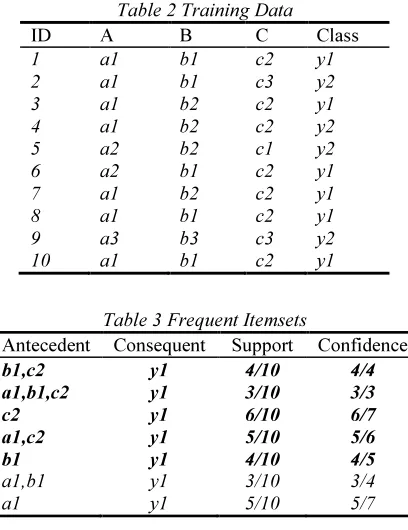
Consider the training data set demonstrated in Table 2 where there are three attributes, A (a1,a2,a3), B(b1,b2,b3) and C(c1,c2,c3), and two classes, y1 and y2. Assuming that the minimum support = 20% and minimum confidence = 80%, the most frequent itemsets are shown in Table 8, together with their supports and confidences. In cases in which an item is associated with multiple classes, only the class with the largest frequency is considered by most of the current AC methods. The frequent items in bold in Table 3 represent those
that passed the confidence and support thresholds and are then converted into rules. Finally, the classifier is constructed using an ordered subset of these rules.
[image:5.595.304.508.419.684.2]AC algorithms frequently experience exponential growth in their number of rules as a result of the association rule discovery approaches, which explore all possible associations between the attribute values in a database. The support threshold is the key to success in both the association rule discovery and AC approaches to data mining. However, for certain application data, some rules with high confidence are ignored simply because they do not have sufficient support. Classic AC algorithms employ one support threshold to control the number of derived rules and may be unable to capture high confidence rules that have low support. To explore a large search space and to capture as many high confidence rules as possible, such algorithms commonly tend to set a very low support threshold, which may give rise to problems such as over fitting. The generation of statistically low support rules and a large number of candidate rules will also cause high CPU time and storage requirements.
Table 2 Training Data
ID A B C Class
1 a1 b1 c2 y1 2 a1 b1 c3 y2 3 a1 b2 c2 y1 4 a1 b2 c2 y2 5 a2 b2 c1 y2 6 a2 b1 c2 y1 7 a1 b2 c2 y1 8 a1 b1 c2 y1 9 a3 b3 c3 y2 10 a1 b1 c2 y1
Table 3 Frequent Itemsets
Antecedent Consequent Support Confidence
b1,c2 y1 4/10 4/4
a1,b1,c2 y1 3/10 3/3
c2 y1 6/10 6/7
a1,c2 y1 5/10 5/6
b1 y1 4/10 4/5
a1,b1 y1 3/10 3/4 a1 y1 5/10 5/7
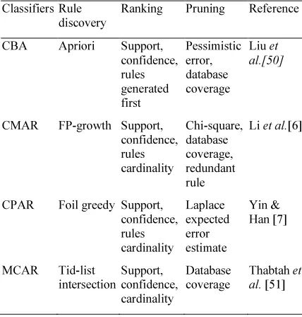
on Association Rule (MCAR) [51]. Those AC varied in several features such as the rules discovery, rank rules and prune rules as noted in Table 4. For the ranking process, researchers have primarily considered support and confidence as the best factors and then followed by their preference measures, in which for pruning measure, database coverage is the most popular. Meanwhile, methods to find CARs are varied such as Apriori, FP-Tree, Foil Greedy and Tid-list intersection. Once the classifier is constructed, its predictive power is evaluated on the test dataset to forecast their class labels.
Table 4 Summary of AC algorithm
Classifiers Rule discovery
Ranking Pruning Reference
CBA Apriori Support, confidence, rules generated first Pessimistic error, database coverage
Liu et al.[50]
CMAR FP-growth Support, confidence, rules cardinality Chi-square, database coverage, redundant rule
Li et al.[6]
CPAR Foil greedy Support, confidence, rules cardinality Laplace expected error estimate Yin & Han [7]
MCAR Tid-list intersection Support, confidence, cardinality Database coverage
Thabtah et al. [51]
2.2 The application of Negative Association Rule in Associative Classification
Recently, the knowledge obtained with NAR has attracted attention from researchers working with AC. While the CBA approach applied PAR to build the classifier, Association Rule Classification with
Positive And Negative (ARC-PAN) [12],
Associative Classifier with Negative rules (ACN) [13] and Multiple Target Negative Target MTNT [52] consider NAR when building the classifier. Table 5 summarizes the main features of the selected methods for discussion. ARC-PAN and ACN are similar in all features compared to MTNT only similar in datasets used which were the UCI datasets. Even though the ARC-PAN and ACN adopted frequent positive for itemset mining, ACN calculated the number of support for each rule
without scanning the database except for the first time while ARC-PAN needed more database scan to obtain the value for support. Therefore, ACN is claimed to have better time in mining CARs compared to ARC-PAN. Meanwhile, MTNT have different features such as the method used and type of NAR. MTNT used exception rule to build a classifier without additional measure for pruning neitherApriori as the basic method for mining rule. MTNT is clearly having more than one target class compared to ARC-PAN and ACN. However, the fundamental process for building classifier is similar to all methods, which is the CBA. Unfortunately, none of the author used generalized negative rule in theirs study.
Table 4 Summary of features negative associative classifiers
Classifiers Methods Additional measures
FIS Approach
ARC-PAN Apriori & CBA
Correlation coefficient
Frequent positive (Support based on database scan) ACN Apriori &
CBA
Correlation coefficient
Frequent positive (Less database scan) MTNT CBA - Frequent positive
(low minimum support)
NAR must be considered in the earliest step of classifier building, the generation of frequent itemsets. The major issue in AC is the discovery of an enormous number of association rules similar to association rule mining. If the classifier uses NAR together with PAR, this issue becomes critical because the number of NAR is far larger than the number of PAR. Therefore, the development of a pruning measure must be a significant area of focus for the researcher to build a classifier with NAR. As for ARC-PAN and ACN, the correlation coefficient threshold was selected for pruning measure in order to eliminate rules that are below the minimum value. In ARC-PAN, the correlation value also indicates the type of rules to mine, either PAR or NAR. If the correlation is negative, NAR will be mined, while if the correlation is positive, PAR will be mined. The correlation coefficient formula is as follows:
(8)
In this equation, Cov(X, Y) represents the covariance of the two variables and σX indicates the standard deviation. The range of values for ρ is
) , ( Y X Y X Cov σ σ
ρ
=
( , )Y X Y X Cov σ σ
ρ
=
( , )between -1 and +1. If the two variables are independent, ρ equals to 0. When ρ = +1, the variables are positively correlated. Similarly, when ρ = −1, the variables are perfectly correlated negatively. A positive correlation is an evidence of the general tendency for the value of Y to
increase/decrease when the value of X
increases/decreases. A negative correlation exists when an increase/decrease in the X value is associated with a decrease/increase in the Y value. However, ACN only prunes NAR compared to ARC-PAN considering both types of rule, NAR and PAR. Finally, a set of significant CARs will be selected to construct the classifier.
ARC-PAN has a major advantage since it is easy to implement but unfortunately the set of CARs generated is not significant enough. Meanwhile, ACN has an advantage of fast mining rules due to the less database scanning. However, the identification of related rules to be considered for calculating support for a particular rule is difficult. MTNT has a disadvantage since it needs more rules to build the classifier. However, the concept is interesting due to the use of exception rule for CARs.
3. FREQUENT POSITIVE ANEGATIVE (FPN) ITEMSET APPROACH
Frequent Positive and Negative Itemset approach used definition 3 in mining negative association rule. FPN still using similar concept of association rule but the support value will also calculate absent item together with present item in the transaction. Let’s describe the concept of an association rule, where I = {i1, i2 ... im} is a set of n distinct items. Let
D be a set of transaction D= {t1, t2, t3, … tn}, tj ⊂ I, where T represents the transaction for a set of items. Let A = {i1, i2, i3, … ik}, A⊂ I, an itemset, be a set of items in I. The association rule takes the form A→B, whereas A⊂ I, B⊂ I and A ∩ B = Ø. Every generated rule has its own measures, support (supp) and confidence (conf). The calculation of support is the frequency of the transaction in D
containing A and B, which is also known as the probability, P(AUB). The value of confidence is the percentage of the transaction in D containing A and also B; this is known as the conditional probability,
P(B|A). The Apriori algorithm uses threshold values to filter the weak and uninteresting rules.
There are two phases in Apriori: the candidate generation phase and rule generation phase, which is also known as the support-confidence framework [3]. The threshold value of the candidate generation phase is the minimum support, whereas the rule
generation phase is the minimum confidence. In the candidate generation phase, itemsets that have greater than the minimum support are called frequent itemsets [FIS], while itemsets that have lower than the minimum support are labelled as infrequent itemsets. In the rule generation phase, frequent itemsets that have greater than the minimum confidence will be employed to generate association rules. In each positive association rule,
A→B can have three forms of NAR: 1) A→¬B; 2)
¬A→B; 3) ¬A→¬B. The Venn diagram for the rule
A→B is as in Figure 1. A∩B is the itemset for generating positive rules while A∩¬B, ¬A∩B and
¬A∩¬B are the itemsets for generating negative rules.
Figure1 Venn diagram for negative and positive rule
Figure 2 The lattice for the negative itemset {A,B,C}
In traditional Apriori, the calculation of support for an itemset is based on the presence of the itemset in the transactions. As an alternative, this paper proposes determining the calculation of support from the absence of items or itemsets for generating NARs, together with the frequent presence of itemset ideas. As a result, the frequent positive and negative (FPN) itemsets will be generated at the end of the candidate generation phase. Figure 3 presents the FPN algorithm that was implemented in this study. Only candidates including the absent itemsets in which the calculated support is above the minimum support value will be extended. For rule generation, we adopted similar steps for those used in the traditional Apriori. All rules with greater than the minimum confidence will be extracted; the rules will consist of PAR and NAR.
For a better understanding of the FPN approach, we conducted a test with a small dataset to illustrate the mining process. Table 6 consists of a transaction dataset, whereas Table 7 shows a frequent itemset that has been discovered. Lk is denoted as all frequent k-itemsets. Table 6 lists all of the generated frequent itemsets, both positive and negative, with minimum support = 0.4. The candidate generation discontinued at L3 because there were no more frequent itemsets with greater than the minimum support. Based on the set of frequent itemsets L3, association rules were generated including both positive and negative rules with minimum confidence = 0.8, as displayed in the right-hand column in Table 8. If we only consider frequent positive (FP) itemsets, item E
will not be considered for NAR mining as in Table 7. As a result, the generated rules will miss out the strongest items in the NARs. Therefore, we diverted from the aim of NAR mining, in which we focused on the absence ofstrong items or itemsets.
Algorithm: Frequent Positive and Negative Itemset (FPN)
Input: D:Transactional Database, ms: minimum support, Ck: candidate itemset of size k, Lk: frequent itemset of size
k
L1-frequent items(l)
Initialize L1, f, countP and countN
scan the database and find the set of items (f) for each item f in F do
for each transaction t ∈ D do
if t contains f then
increment the count of countP; else
increment the count of countN; if countP≥ms or countN≥ms L1← L1 {f}
return L1
For(k=1; Lk!=Ø; k++) do begin
Ck+1=candidates generated from Lk;
For each transaction t in D do
Increment the count of all candidates in Ck+1 are contained in t
Increment the count of all candidates in Ck+1 are
not contained in t
Lk+1=candidates in Ck+1 with ≥ ms
Return kLk
Figure 3 FPN Algorithm
Table 6 Transaction Data
TID Items
1 A,B,D
2 A,B,C,D
3 B,D
4 B,C,D,E
5 A,C,E
6 B,D,F
7 A,E,F
8 C,F
9 B,C,F
10 A,B,C,D,F
Table 7 Frequent Itemsets (FIS)
L1 Supp
A 5
¬A 5
B 7
C 6
¬C 4
D 6
¬D 4
¬E 7
F 5
¬F 5
L2 Supp
¬A^B 4
¬A^¬E 4
B^C 4
B^D 6
B^¬E 6
B^¬F 4
C^¬E 4
D^¬E 5
D^¬F 4
¬E^F 4
L3 Supp
B^D^¬E 5 B^D^¬F 4
frequent present itemsets. There are only two frequent positive itemsets in L2, whereas there are eight frequently negative itemsets. When those frequent itemsets went through the rules generation phase, 16 rules were generated: 14 rules are NAR and only two rules are PAR. Furthermore, the generated NARs are strong and considered interesting as demonstrated in Table 8 by the values of the confidence and support. Those rules are vital and should be considered in the process of analysis to improve classification task or decision-making.
Table 8 Association Rules
Frequent +ve Frequent +ve & -ve
D→B {100, 6} B^¬F→D {100,5} D^¬F→B {100,4} B→D {85,6} ¬A→B {80,4} ¬F→B^D {80,4} ¬F→D {80,4}
D→B {100, 6} B^¬F→D {100,5} D^¬F→B {100,4} B→D {85,6} ¬A→B {80,4} ¬F→B^D {80,4} ¬F→D {80,4} D^¬E→B {100,5} B→¬E {85,6} ¬E→B {85,6} D→¬E {83,5} D→B^¬E {83,5} B^¬E→D {83,5} B^D→¬E{83,5} ¬F→B {80,4} F→¬E {80,4}
We also evaluated the generated rules with selected measures such as interest [32], Piatetsky Shapiro [50] and collective strength [51] as presented in Figure 4, and the results are encouraging. The selected measures are commonly used for association rule mining. Those measures are succeeding to achieve their objectives and the values added to the traditional measures include support and confidence.
a)Interest (I) [6]: To find the dependence of items, in order to determine the cause of the correlation. The further the value from 1, there will be more dependence between the items. Interest values above 1 indicate positive dependence, while those below 1 indicate negative dependence. Interest values = 1 indicate that the two sets are independent. The interest measure is preferable as it directly captures correlation, as opposed to confidence which considers the directional implication (and treats the absence and presence of attributes non-uniformly). The formula of interest is as in Equation (9).
) ( ) ( ) ( B P A P AB P
I= (9)
b)
c)Collective Strength (CS) [2]: The collective strength of an itemset is defined as a number between 0 to ∞ and the Equation as in (10). A value of 0 indicates aperfect negative correlation, while a value of ∞ indicates a perfect positive correlation. A value of 1 indicates the “break-even point”, corresponding to an itemset present at the expected value. An itemset is said to be in violation of a transaction, if some of the items are present in the transaction while others are not. Thus, the concept of violation denotes how many times a customer may buy at least some of the items in the itemset, but may not buy the rest of the items.
) ( ) ( 1 ) ( ) ( ) ( ) ( 1 ) ( ) ( ) ( ) ( ) ( ) ( A B P AB P B P A P B P A P B P A P B P A P A B P AB P CS ¬ ¬ − − ¬ ¬ − − × ¬ ¬ + ¬ ¬ + (10)
d)Piatetsky Shapiro (PS) [8]: This measure which is a formula in Equation (11) has three principles that should be obeyed by good measures such as below:
• F = 0 if A and B are statistically independent,
that is, P(AB) = P(A)P(B).
• F monotonically increases with P(AB) when
P(A) and P(B) remain the same.
• F monotonically decreases with P(A) (or P(B))
when P(AB) and P(B) (or P(A)) remain the same.
PS = P(AB) − P(A)P(B) (11)
All values as in Figure 4 are the average values for each measure of all selected rules. FPN (continuous line) is dominant in almost all measures compared to FIS (broken line) except in the interest and collective strength values. However, the differences are very slim, 0.02 and 0.15 respectively. Most importantly, FPN successfully mines the number of strong NAR two times more compared to FIS approach. Therefore, mining from FPN itemsets is expected to discover interesting NARs. Consequently, an optimum number of strong and interesting NARs and PARs will be discovered at the end of the rule generation phase as we focused on itemsets that have a high frequency of absence or presence.
4. FPN-AC CLASSIFIER
In this paper, we proposed a new classifier and named it as FPN-AC. FPN-AC is the application of the FPN itemset approach in AC. Figure 5 indicates the steps used in the FPN-AC approach, which begin with training data to learn the hidden pattern and build the classifier. The algorithm version of FPN-AC is as in Figure 6. The steps are adapted from CBA [45] and can be divided into five main steps. The FPN approach is embedded in the first and second steps to prune weak rules together with interest measure. As a result, interesting CARs will be generated for consideration to build classifier.
• Step 1: The discovery of all frequent itemsets
with FPN approach.
• Step 2: The pruning strategy for frequent itemsets
to generate CARs.
• Step 3: The selection of one subset of CARs to
form the classifier.
• Step 4: The ranking solution for CARs in the
classifier.
• Step 5: Evaluating the accuracy of the classifier
[image:10.595.301.510.83.345.2]on the test data.
Figure 5 Diagram for the proposed FPN-AC
Input: D // the transaction database
ms // user defined threshold for the minimum support
mc // user defined threshold for the minimum confidence
intr // user defined threshold for the minimum interest
Output: C // classifier consists of selected rule and default class
accuracy of C //indicates the accuracy of classifier
Mining the FPN items on database D using ms
Pruning the FPN itemsets on database D using intr Generating rules from FPN itemsets
Selecting rules to form classifier using mc R = sort(R);
for each rule r ∈R in sequence do
temp = Ø;
for each case d ∈D do
if d satisfies the conditions of r then
store d.id in temp and mark r if it correctly classifies d;
if r is marked then insert r at the end of C;
delete all the cases with the ids in temp from D;
selecting a default class for the current C; compute the total number of accuracy of C; Find the first rule p in C with the lowest total number of errors and drop all the rules after p in C;
Add the default class associated with p to end of C, and return C (our classifier).
Figure 6 FPN-AC Algorithm
a)Step 1
The function of FPN is to select frequent items in which there are more than the minimum support values, whether in terms of the positive (for PAR) or negative (for NAR) of the item. On the other hand, both ARC-PAN and ACN adopted a similar FIS concept used in the Apriori algorithm but the steps for generating FIS are based only on the frequent positive of items. The beginning stage is the most challenging; it is computationally expensive because the mining space for FIS is enormous, especially with high-dimensional data.
b)Step 2
The number of rules generated from the FPN process is still huge. Therefore, the pruning measure is conducted in phase 2, which uses interest measure as in Equation (3). The weak itemsets will be eliminated by measuring their correlations or interest, which are below the minimum interest value whether from a frequent absence or frequent presence of the itemset. The objective of these measures is to eliminate uninteresting rules and focus on interesting rules by setting a certain value so that decisions can be made quickly according to the rules. More importantly, the mining space will be reduced for exploring strong CARs.
c)Step 3
[image:10.595.94.298.410.555.2]and a confidence value less than the minimum confidence threshold.
d)Step 4
At the end of phase 2, strong CARs will be ready for use in the building of the classifier. However, the selected CARs need to be ranked according to their strengths so that the strongest rule will be chosen to be tested first. The ranking solution is adopted from CBA, for two rules, ri and rj, where ri precedes rj by following several rules:
• Rule 1: The confidence or ri is greater than that of rj,
• Rule 2: Their confidences are the same, but the
support of ri is greater than that of rj, or
• Rule 3: Both the confidence and supports of ri and rj are the same, but ri is generated earlier than rj.
e)Step 5
The final step is the evaluation of the classifier using the testing data, in which after a set of rules is generated and ranked, an evaluation step takes place to test each rule in order to remove redundant rules. If a rule correctly classifies at least a single instance, it will then be a potential rule in our classifier. In addition, all instances correctly classified by it will be deleted from the training data. In a case that a rule has not classified any training instance, it will then be removed from the rules set. A default class is also chosen (the majority class in the remaining data), in which means that if we stop selecting more rules for our classifier this class will be the default class. We then compute and record the total number of errors that are made by the current and default class. This is the sum of the number of errors that have been made by all the selected rules in classifier and the number of errors to be made by the default class in the training data. When there is no rule or training case left, the rule selection process is completed. Discard those rules that do not improve the accuracy of the classifier. The first rule at which there is the least number of errors recorded is the cut off rule. All the rules after this rule can be discarded because they only produce more errors. The undiscarded rules and default class of the last rule from the classifier.
5. EXPERIMENTAL RESULTS AND DISCUSSION
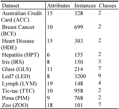
We conducted experiments on eleven different datasets from the UCI Machine Learning Repository [52]. Table 8 presents the main features
[image:11.595.306.507.327.511.2]of selected datasets. A stratified 10-fold cross validation was performed on each dataset to evaluate the performance of the classification algorithms and to evaluate the accuracy of the learning technique. Stratification entails proper representation of each class in both the training and test datasets following the sampling procedure by random sampling of the dataset when performing the 10-fold partitions. To provide a fair comparison with other algorithms, we used the same discretisation method employed by Liu et al.[45], which uses the Entropy method described by Fayyad and Irani [53]. We also adopted the same threshold values used in previous research for fair benchmarking: 1% for minimum support and 50% for minimum confidence.
Table 8 Datasets Description
Dataset Attributes Instances Classes
Australian Credit Card (ACC)
15 328 2
Breast Cancer (BCE)
10 699 2
Heart Disease (HDE)
15 303 2
Hepatitis (HPT) 6 155 2
Iris (IRS) 8 150 3
Glass (GLS) 11 214 7
Led7 (LED) 8 3200 9
Lymph (LYM) 19 148 4
Tic-tac (TTC) 10 958 2
Pima (PIM) 9 768 2
Zoo (ZOO) 18 101 7
FPN-AC. As demonstrated in Table 9, the results for accuracy based on the FPN method are very encouraging. The results of classification accuracy for FPN-AC are higher than those of other classifiers in the majority of datasets. As seen in Table 9, the wins/ties/lossess record of FPN-AC against other classifiers is 9-0-2. In particular, in the HDE dataset, the accuracy is more than 10% greater than those of other classifiers. In contrast, the accuracy for the LED dataset is the lowest among the classifiers, due to the higher number of class in LED dataset compared to other datasets. An examination of the results of our experiment shows that the performance of the classifier decreases when the number of classes in each dataset increases.
Table 9 Classifier accuracy for C4.5, CBA, ARC-PAN, ACN and FPN-AC
Datasets C4.5 CBA ARC-PAN
ACN FPN-AC
ACC 86.5 86.4 - 85.5 93.2W
BCE 96.1 95.8 96.2 95.3 97.8 W
HDE 81.1 81.5 83.8 82.2 96.8 W
HPT 77.4 84.9 - 83.2 90.4 W
IRS 94.7 92.9 94.0 95.3 99.0 W
GLS 72.5 72.6 - - 76.5 W
LED 73.5 72.2 71.1 71.9 57.1L
LYM 79.0 80.4 - 83.1 91.8 W
TTC 99.4 100.0 - 99.7 100.0 W
PIM 72.5 72.4 73.1 76.3 89.2 W
ZOO 92.2 94.6 - - 92.0 L
SIG 0.09 0.12 0.39 0.47
The symbols W/T/L indicate the wins, ties or losses.
We also observe that the number of CARs and number of rules in classifier for FPN-AC (broken line) are less compared to CBA (continuous line), as shown in Figure 7 (a) and (b), respectively, due to the smaller number of frequent itemsets (FIS) generated by FPN-AC. Therefore, the mining space is smaller and the processing time is definitely reduced. This efficiency is only achieved when the pruning factor is imposed, which is an interest measure without risking the classifier accuracy. The optimum number of rules in the classifier is also important for obtaining a higher quality classifier. If the number of rules is too high, the high coverage may come at the sacrifice of having a lower number of correct rules and consequent reduction in accuracy. If the number of rules in the classifier is too small, an insufficient number of rules will be used for classification, thereby decreasing the
accuracy value. A small number of classification rules is desirable, especially when the rules are strong, to enable a more rapid classification phase. Furthermore, a small set of rules is easier to comprehend and manage. Nevertheless, FPN-AC has better accuracy in themajority of datasets as in Figure 7 (c).
(a)
(b)
(c)
Figure 7 Comparison of number of CARs (a), number of rules (b) and accuracy (c)
The comparison between the negative associative classifiers in Table 10 reflects that FPN-AC still achieve better accuracy than ARC-PAN and ACN. However, we can only compare some of the datasets because the accuracies of ARC-PAN and ACN were only available for some of the datasets. It is clear that FPN successfully avoids the loss of knowledge or incomplete knowledge that can lower the accuracy of the classifier. In addition, FPN is able to obtain important knowledge for an accurate classifier. It is clear from the results that AC is superior to the state-of-the-art classification algorithm C4.5. A statistical t-test was performed to measure the significance of the difference in performance results between FPN-AC and the
[image:12.595.95.281.340.510.2]comparative methods (C4.5, CBA, ARC-PAN and ACN) in relation to the classification accuracy. Table 10 also denotes the significant differences between FPN-AC versus C4.5, FPN-AC versus CBA, FPN-AC versus ARC-PAN and FPN-AC versus ACN, as shown in the row entitled SIG. The difference in the performance of FPN-AC versus C4.5 had a p-value of 0.09, which is slightly closer to the p value of 0.05, which indicates that the methods are considered comparable in terms of performance. Similarly, comparison of the results of FPN-AC versus those of other methods resulted in p values of higher than 0.05, indicating that other relevant methods are also considered comparable in terms of performance. In addition, the p value for the comparison of FPN-AC and CBA is lesser, 0.12, which is more significant than the differences between ARC-PAN, 0.39, and ACN, 0.47.
6. CONCLUSION
The aim of this research is to improve the classification accuracy using FPN itemset approach to generate the NAR. It is essential that thestrong NAR is selected for CARs to build an accurate associative classifier. A naive approach to generatingNAR would create a very large number of rules. In addition to the generation of a large number of rules, many of the rules may be of low interest. We have devised an enhanced algorithm for NAR generation, which is different from other algorithms in the sense that it considers the frequently absent itemsets together with frequent present itemsets. Although the mining space is greater, the hidden knowledge is crucial especially for critical data or domain. Therefore, FPN-AC also adopted interest as pruning measure to eliminate unimportant itemsets in mining NAR. This research also approaches the problem of generating NAR from a classification perspective, considering methods of generating a sufficient number of high-quality CARs to enhance theclassification accuracy and speed up the classification process. This research demonstrated that the knowledge obtained from the strong NAR produced from FPN offers an advantage to the classification task by providing higher accuracy classifier.
REFRENCES:
[1] J. Han, M. Kamber, and J. Pei, Data mining: concepts and techniques: Morgan Kaufmann Pub.
[2] R. Srikant and R. Agrawal, "Mining quantitative association rules in large relational tables," in SIGMOD, 1996, pp. 1-12.
[3] C. C. Aggarwal and P. S. Yu, "A new framework for itemset generation," in ACM SIGACT, 1998, pp. 18-24.
[4] R. Agrawal and R. Srikant, "Fast algorithms for mining association rules," in Very Large Data Bases, 1994, pp. 487-499.
[5] Z. Tang and Q. Liao, "A new class based associative classification algorithm," International Journal of Applied Mathematics, 2007.
[6] W. Li, J. Han, and J. Pei, "CMAR: Accurate and efficient classification based on multiple class-association rules," in ICDM, 2001, pp. 369–376.
[7] J. Yin and X. Han, "CPAR: Classification based on predictive association rules," in SIAM, 2003, p. 331.
[8] Y. Lan, D. Janssens, G. Chen, and G. Wets, "Improving associative classification by incorporating novel interestingness measures," Expert Systems with Applications, vol. 31, pp. 184-192, 2006.
[9] E. Baralis and P. Garza, "A lazy approach to pruning classification rules," in ICDM, 2002, pp. 35-42.
[10] F. Thabtah, "Rules pruning in associative classification mining," in IBIMA 2005, pp. 7-15.
[11] Y. Zhao, H. Zhang, S. Wu, J. Pei, L. Cao, C. Zhang, and H. Bohlscheid, "Debt Detection in Social Security by Sequence Classification Using Both Positive and Negative Patterns," Machine Learning and Knowledge Discovery in Databases, pp. 648-663, 2009.
[12] M. L. Antonie and O. R. Zaïane, "An associative classifier based on positive and negative rules," in ACM SIGMOD 2004, pp. 64-69.
[13] G. Kundu, M. M. Islam, S. Munir, and M. F. Bari, " ACN: An Associative Classifier with Negative Rules," in Science and Engineering, 2008, pp. 369-375.
rules," Knowledge and Information Systems vol. (2005) 7, pp. 158-178, 2004.
[15] Y. S. Koh and R. Pears, "Efficiently Finding Negative Association Rules Without Support Threshold," AI, LNAI 4830, pp. 710-714, 2007. [16] P. K. Bala, "A technique for mining negative association rules," in Proceedings of the 2nd Bangalore Annual Compute 2009, pp. 1-4. [17] M. L. Antonie and O. R. Zaïane, "Mining
positive and negative association rules: An approach for confined rules," Knowledge Discovery in Databases: PKDD 2004, pp. 27-38, 2004.
[18] Y. Ben-Gang and C. Li, "A Novel Mining Algorithm for Negative Association Rules," in Intelligent Systems, 2009, pp. 553-556.
[19] H. Jiang, Y. Zhao, and X. Dong, "Mining Positive and Negative Weighted Association Rules from Frequent Itemsets Based on Interest," in Computational Intelligence, 2008, pp. 242-245.
[20] L. Zhou and S. Yau, "Efficient association rule mining among both frequent and infrequent items," presented at the Computers & Mathematics with Applications, 2007.
[21] H. Zhu and Z. Xu, "An effective algorithm for mining positive and negative association rules," in Computer Science and Software Engineering, 2008, pp. 455-458.
[22] X. Yuan, B. P. Buckles, Z. Yuan, and J. Zhang, "Mining negative association rules," in Proceedings of the Seventh International
Symposium on Computers and
Communications (ISCC’02), 2002, pp. 623-628. [23] S. T. Dongme Sun, Wei Zhang, Haibin Zhu, "An Algorithm to Improve the Effectiveness of Apriori," in Proc. 6th IEEE Int. Conf. on Cognitive Informatics (ICCI'07), 2007.
[24] S.-C. C. Liewean Cheng, And Jashen Chen, "Applying Weighted Association Rules with the Consideration ofProduct Item Relevancy," in IEEE, 2009, pp. 888-893.
[25] X. F. Jianhua Liu, Zhihua Qu, "A New Interestingness Measure of Association Rules," presented at the Second International Conference on Genetic and Evolutionary Computing, 2008.
[26] L. H. Yu Zhefu, "A New Association Rule for Causes and Effects Analysis," presented at the 2009 International Joint Conference on Artificial Intelligence, 2009.
[27] Z. L. Huan Wu, Lin Pan, Rongsheng Xu, Wenbao Jiang, "An Improved Apriori-based Algorithm for Association Rules Mining," presented at the Sixth International Conference on Fuzzy Systems and Knowledge Discovery, 2009.
[28] H. Z. Gang Yang, Lei Wang, Ying Liu, "An
Implementation of Improved Apriori
Algorithm," presented at the Proceedings of the Eighth International Conference on Machine Learning and Cybernetics, Baoding, 2009. [29] L. Ji, B. Zhang, and J. Li, "A New Improvement
on Apriori Algorithm," presented at the Computational Intelligence and Security, 2006. [30] Y. L. Yiwu Xie, Chunli Wang, Mingyu Lu,
"The Optimization and Improvement of the Apriori Algorithm," presented at the International Symposium on Intelligent
Information Technology Application
Workshops, 2008.
[31] Z.-P. L. Wei-Min Ma, "Two Revised Algorithms Based On Apriori for Mining Association Rules," in Proceedings of the Seventh International Conference on Machine Learning and Cybernetics, Kunming, 2008, pp. 350-355.
[32] S. Brin, R. Motwani, and C. Silverstein, "Beyond market baskets: Generalizing association rules to correlations," ACM SIGMOD Record, vol. 26, pp. 265-276, 1997. [33] T. Ma, J. Leng, M. Cui, and W. Tian, "Inducing
positive and negative rules based on rough set," Information Technology Journal, vol. 8, pp. 1039-1043, 2009.
[34] D. T. Olena Daly, "Exception Rules Mining Based on Negative Association Rules," presented at the ICCSA 2004, LNCS 3046,, 2004.
[35] X. Wu, C. Zhang, and S. Zhang, "Efficient mining of both positive and negative association rules," ACM Transactions on Information Systems (TOIS), vol. 22, pp. 381-405, 2004. [36] C. Cornelis, P. Yan, X. Zhang, and G. Chen,
"Mining positive and negative association rules from large databases," in Cybernetics and Intelligent 2006, pp. 1-6.
[38] F. Hussain, H. Liu, E. Suzuki, and H. Lu, "Exception rule mining with a relative interestingness measure," Knowledge Discovery and Data Mining. Current Issues and New Applications, pp. 86-97, 2000.
[39] W. G. Teng, M. J. Hsieh, and M. S. Chen, "A statistical framework for mining substitution rules," Knowledge and Information Systems, vol. 7, pp. 158-178, 2005.
[40] A. Savasere, E. Omiecinski, and S. Navathe, "Mining for strong negative associations in a large database ofcustomer transactions," in Data Engineering, 1998, pp. 494-502.
[41] X. Peng and Y. Wu, "Research and application of algorithm for mining positive and negative association rules," in Electronic and Mechanical Engineering and Information Technology, 2011, pp. 4429-4431.
[42] S. Tsumoto, "Mining Positive and Negative Knowledge in Clinical Databases Based on Rough Set Model," presented at the PKDD 2001, LNAI 2168, 2001.
[43] O. Daly and D. Taniar, "Exception Rules Mining Based on Negative Association Rules," presented at the ICCSA 2004, LNCS 3046,, 2004.
[44] H. Jiang, Y. Zhao, C. Yang, and X. Dong, "Mining Both Positive and Negative Weighted Association Rules with Multiple Minimum Supports," in Computer Science and Software Engineering, 2008, pp. 407-410.
[45] Y. Zhao, H. Zhang, L. Cao, C. Zhang, and H. Bohlscheid, "Mining both positive and negative
impact-oriented sequential rules from
transactional data," Advances in Knowledge Discovery and Data Mining, pp. 656-663, 2009. [46] H. Jiang, X. Luan, and X. Dong, "Mining
Weighted Negative Association Rules from Infrequent Itemsets Based on Multiple Supports," in Industrial Control and Electronics Engineering (ICICEE), 2012 International Conference on, 2012, pp. 89-92.
[47] X. Dong, S. Wang, H. Song, and Y. Lu, "Study on negative association rules," Transactions of Beijing Institute of Technology, vol. 24, pp. 978-981, 2004.
[48] F. A. Thabtah, "A review of associative classification mining," The Knowledge Engineering Review, vol. Vol. 22:1, pp. 37-65, 2007.
[49] E. Suzuki, "Discovering interesting exception rules with rule pair," in PKDD workshop on advances in inductive rule 2004, pp. 163-178. [50] B. Liu, W. Hsu, and Y. Ma, "Integrating
classification and association rule mining," Knowledge Discovery and Data Mining, pp. 80–86, 1998.
[51] F. Thabtah, P. Cowling, and Y. Peng, "MCAR: multi-class classification based on association rule," in Computer Systems and Applications, 2005, p. 33.