10
EMPIRICAL EVALUATION OF DIFFERENT CLUSTERING
APPROACHES FOR VISUAL CODEBOOK GENERATION
1JURAJ RABCAN, 2GABRIELA GRMANOVA
1,2
Slovak University of Technology, Faculty of Informatics and Information Technologies, Institute of
Informatics and Software Engineering
E-mail: [email protected], [email protected]
ABSTRACT
Bag of Visual Words is a common representation of images in computer vision. The important task for this representation is a creation of visual codebook, where the set of all considerable visual words is stored. Visual words are represented by descriptors of local features and to reduce their amount and to choose only significant ones, the visual codebook is generated by clustering of these descriptors. State of the art for clustering descriptors of local features is menas algorithm. The drawback of codebook generation by k-means algorithm is that cluster centers are located in high density areas. In this paper, we investigate several other algorithms and we compare them with k-menas algorithm. Tested algorithms are similar to k-means in their goals, but have algorithmically different approaches. Comparison is done by evaluating of image retrieval task on UK-bench dataset and classification on Caltech 101.
Keywords: Bag of Visual Words, Clustering, Local features, Image retrieval
1. INTRODUCTION
Systems for searching and indexing text documents are nowadays considered as mature and so effective that they can operate with millions of files at once. A common representation of documents in this field is called Bag of Words. Text documents are represented by a set of words and phrases occurring in the documents. This set can be stored as feature vectors, which represent documents by their word counts (histogram of word occurrences in the document). Since the occurrence of a given word tends to be sparse across different documents, one can create a query based on keywords, which produce relevant content in real time.
In computer vision, a representation of images, inspired by Bag of Words, is named Bag of Visual Words. Visual words represent the analogy to words from text documents, and they represent small parts of the images that carry some kind of information. This representation is popular in the field of image retrieval systems. Bag of Visual Words rely on a visual codebook. It is a vocabulary where all visual words from the documents are stored and it can be generated by clustering descriptors of local features. Cluster centers are then considered to be visual words. Codebook generation is one of the most important steps in the tasks where the Bag of Visual Words is used, since
a proper creation of the codebook can increase within-class and between-class discriminative power of a system.
Until now, many approaches for visual codebook creation were presented [1,2,3]. The quality of the visual codebook has a significant impact on the success of a method that uses visual codebook. The clustering is a central task for codebook generation and there were developed many clustering algorithms. State of the art algorithm for codebook generation is the k-means algorithm. The drawback of k-means is that it sets the most of the cluster center points near to very dense areas [3]. Furthermore, k-means is not deterministic algorithm, so it is necessary to run learning process multiple times. As an alternative to k-means algorithm, there can be used one of many other clustering algorithms, each having different properties. The existence of different alternatives to k-means algorithm led us to apply several selected algorithms in the process of visual codebook generation.
11 clustering descriptors of local features. Section 6 deals with the introducing of experiments performed on the datasets. Section 7 deals with the summary of obtained results. In Section 8 one can find the discussion about obtained results and used algorithms. Section 9 concludes with future direction of work and short summary of obtained results.
2. LOCAL FEATURES
Local features are crucial for the Bag of Visual Words representation because visual words are obtained by their clustering. Commonly used algorithm for detecting local features is the SIFT (Scale Invariant Feature Transform) algorithm. It has two phases, where in the first phase key-points are detected and in the second phase local descriptors are computed. This method was introduced by David Lowe in [4], but great response was caused by the paper [5] by the same author.
The first step of key-points detection is a creation of scale pyramid. The scale pyramid is made by rescaling of the picture to many scales - octaves. At every octave, a picture is blurred several times. Blurring operation is realized by convolution with the Gaussian kernel:
L x, y,σ I x, y ∗ G x, y,σ ,
where L is the blurred image, I is the original image, σ is the blurred factor and G is the Gaussian kernel defined as follows:
1 2
Once the scale pyramid is created, key-points can be detected by Difference of Gaussians - DoG. DoG is applied on neighboring images from every octave as follows:
D x, y,σ G x, y, kσ x, y,σ ∗ ,
x, y, kσ x, y,σ ,
where k is the blurred factor between two neighboring images. When DoG is done, pixel whose all neighboring pixel values are smaller or greater than values of evaluated pixel are then considered to be key-points. Some filters can be applied to reduce amount of points i.e. key-points lying on lines can be filtered [6].
The next step of SIFT method is the creation of local descriptors for the detected key-points. Local descriptors describe the key-point’s neighborhood. Those descriptors should be invariant against scale changes, affine distortions
or changes in illumination. SIFT descriptors are computed from circular region around the key-point, which is divided into 4 × 4 not overlapping patches.
SIFT descriptor of a given key-point is the histogram of gradient orientations within the patches. Each patch is sampled by 16 points Lxy and for each point the size mxy and the orientation of gradient θxy a r e c o m p u t e d as follows:
!"# $ "%&,# ' &,( )* ",#%& ",# & )
+"# ,-. &
",#%& ",# &
"%&,# ' &,(
Each key-point histogram has a dimensionality 128 (8 patches × 16 gradient orientations).
As an alternative to SIFT, there is a lot of different methods. Widely used is SURF [7] and ORB [8], but recent studies [9] have shown that SIFT is the best known option to calculate descriptors because it is invariant to scale and rotation and it is partially invariant to change in illumination and 3D camera viewpoint too.
3. VISUAL CODEBOOK
Visual codebook represents the vocabulary of all visual words which can occur in the documents. Each descriptor of local feature is labeled according to the most similar visual word from the codebook. As mentioned before, it is created by clustering the descriptors of local features. Many algorithms for clustering (including k-means) need to set the number of clusters as an input parameter. It is not easy to say how many clusters is needed, because it is not known how many visual words occur in the dataset. Thus, when using the algorithm that needs to know the number of clusters in advance, the clustering must be done several times with different number of clusters to discover the suitable value. Creating of visual codebook can be briefly described by 3 steps:
1. key-points detection,
2. key-points descriptors for the whole dataset computation,
3. descriptors clustering.
12
Figure 1: Illustration of creating visual codebook
4. BAG OF VISUAL WORDS
In Bag of Visual Words representation, the image is represented as a histogram of visual words from the image. This representation is popular in image retrieval systems and in object recognition tasks. Since key-points, local descriptors and visual codebook are explained above, we can show how the Bag of Visual Words representation can be derived for a single image:
1) Key-points detection for input image 2) Computation of descriptor for each
detected key-point
3) Labeling every descriptor by the visual word representing the nearest cluster 4) Creating histogram of the labels
4.1 Tiling method
[image:3.612.139.251.639.697.2]The drawback of Bag of Visual Words representation is that it completely ignores spatial information among visual words. To solve this drawback, tiling method [10] has been used in our experiments. According to the mask, an image is partitioned into several tiles. For every tile, a histogram of visual words is created. Image is then represented by concatenated histograms of visual words from all tiles. An example of the mask is illustrated in Figure 2.
Figure 2: Illustration of tiling mask which has been used in all our experiments
5. CLUSTERING
The most common algorithm for clustering of local feature descriptors is k-means [11]. For codebook generation was k-means used in many works, e.g. [1,5,12]. The drawback of codebook generation by k-means algorithm is that cluster centers are located only in high density areas. Due to this problem, the Bag of Visual Words models were introduced with different clustering algorithms i.e. online mean-shift algorithm [2] or hierarchical clustering forest [13]. In this paper we evaluate Bag of Visual Words model for image retrieval and classification task. We apply different clustering algorithms as the alternatives to the k-means and we evaluate how these algorithms impact the image retrieval and the classification results. In our experiments, we evaluate the clustering algorithms that use different approaches. Algorithms Mean-shift and DBSCAN are density based, BIRCH is hierarchical algorithm, k-means belongs to partitioning algorithms and self-organizing map is a type of neural network.
A. K-means
K-means algorithm [11] has become a frequently used algorithm in the process of creation of visual codebooks. It is also known as Lloyd’s algorithm, according to its author. The aim of the algorithm is to split instances into clusters, where each instance is assigned to the nearest cluster center.
The algorithm converges to a local minimum, thus it may not find the global optimal solution. The algorithm is sensitive to initialization, so it is necessary to run it several times. The steps of the algorithm are described briefly as follows:
1) From the set of clustering objects randomly choose / instances. These randomly selected instances represent cluster center.
2) All objects 0 are assigned to the cluster, with the nearest cluster center. Thus, 0 is assigned to the cluster 12, where:
j arg !7. d 0, 19
9
13 cluster center and the objects belonging to the cluster:
c= N ? x1 @, ∀x@ ∈ C=
DE
@F&
3) Repeat step 2 and 3 until the stopping condition is satisfied.
B. Self-organizing map
Self-organizing map is a type of neural network which can be used for data clustering. Self-organizing maps are widely used in many areas i.e. collaborative filtering [14] or in gene analyses [15].
The goal of self-organizing map is to find a set of centroids and assign each object from the dataset to the closest centroid. In neural network terminology neurons can be seen as analogous to centroids. Self-organizing map consists of two layers. An input layer projects vectors from training dataset to the grid of neurons. Similar input vectors cause a response on neurons which are physically near in the grid [16]. Widely used algorithm for training of Self-organizing map is Kohonen’s algorithm [16]. The steps of the algorithm can be described briefly as follows:
1) Initialize neuron’s weight vectors. Initialization is done by randomly selected input vectors.
2) Randomly select an input vector x, and find the winner neuron
7
∗ for selected input vector:7∗ arg !7. d
G x, H0
0
where IJis a distance measure function, is an input vector and wi is t h e weight vector.
3)
Update weight wi vector of the winner neuron and his neighbors:H0 , * 1 H0 , * K , . M 7, 7∗ . N , H7 , O,
where parameter K is the learning rate, M 7, 7∗ is the neighborhood function and t is
the number of epochs. Learning rate and size of neighborhood are gradually decreased.
4)
Repeat step 2 and 3 until the stopping condition is satisfied.When the self-organizing map is trained, we perform means clustering where input fork k-means is the SOM grid. When clustering is done neurons are labeled and can be considered to be analogy of the visual words. The reason why k-means is used for labeling grid is that topological near neurons are labeled with the same label and then topology of neurons is preserved in the histograms of visual words.
C. BIRCH
BIRCH algorithm [17] is designed for very large datasets. Birch scans the dataset only once, what dramatically reduces the overhead needed to access data on the disk. The idea of the algorithm is based on the clustering subclusters instead of performing the clustering on individual instances. The core of BIRCH algorithm is the CF tree, which is characterized by CF features. CF feature maintains t h e information about t h e cluster. It is formally defined as triplet CF = (N, LS, SS), where N is the number of instances in the cluster. LS is a linear sum of instances in t h e cluster:
P ? x@,
DE
@F&
where @ is the i-th instance from the cluster. SS is the square sum:
PP ? x)@,
DE
@F&
CF tree is then a high balanced tree, which carries information about t h e clusters. To create CF tree, we need to set two parameters - the branching factor (F,L) and the threshold P. Inner node of the CF tree may contain at most F instances and each leaf node m a y contain at most L instances. Diameter of each node may be less than d e fi ned threshold P.
14 cluster and CF features of visited nodes are updated. If the threshold rule is violated, than a new cluster with corresponding leaf node is created and CF features of visited nodes are updated.
D. DBSCAN
DBSCAN [18] is a density based clustering algorithm. The algorithm clusters samples by growing high density areas, and it can find any shape of the cluster. DBSCAN requires two parameters ε and P. ε represents a radius of a sample and P is the minimal number of samples in one cluster. Clustering process starts in a starting point x that has not been visited. If the number of neighboring samples of x in a shorter distance than ε is greater than parameter P, then a new cluster is formed. The cluster is created by the point x and all his neighbors. The process is recursively repeated for all not visited points belonging to the cluster. If a cluster is fully expanded (all possible points for the cluster are visited), then the algorithm proceeds to iterate over the remaining unvisited samples that are not assigned to any cluster.
DBSCAN is able to detect the noise samples. If the number of neighboring samples is smaller than P, then point x is considered to be the noise. The advantage of DBSCAN is in its ability to determine the number of clusters. The disadvantage of the algorithm is its inability to cluster the datasets having clusters with varying densities. DBSCAN finds clusters of arbitrary shape. It can even find clusters completely surrounded by another cluster. Because of its ability to find clusters of arbitrary shapes, the cluster cannot be represented by the centroid or medoid. To find such a representative of each cluster, some kind of a classifier can be adopted.
E. Mean-shift
Mean-shift algorithm [19] is widely used in texture segmentation and object tracking tasks, but it can be used for clustering of any kind of data. This method does not require to predetermine the number of clusters.
Similarly to DBSCAN, mean-shift is a density based algorithm. For density estimation the algorithm uses so-called kernel. Kernel is defined by its position and radius. Its role is in finding the center of a cluster. The kernel is moving to the space with the highest density of points in the area. The shift amount and direction is determined from the center of gravity of the points in the kernel.
T he kernel is repeatedly shifted to the position, such that the center of gravity is in the middle of the kernel.
[image:5.612.316.512.189.234.2]The advantage of this algorithm is that it is fully deterministic. On the other hand, the disadvantage is in its time complexity. The idea of this algorithm is illustrated in Figure 3.
Figure 3: Illustration of Mean-shift on 2D dataset.
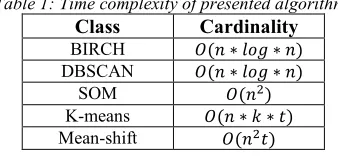
5.1 Time complexity of presented algorithms
The time complexity of the presented algorithms can be seen in the Table 1, where . the number of samples is, / is the number of clusters and t is the number of iterations.
Table 1: Time complexity of presented algorithms
Class Cardinality
BIRCH Q . ∗ RST ∗ . DBSCAN Q . ∗ RST ∗ .
SOM Q .)
K-means Q . ∗ / ∗ , Mean-shift Q .),
Algorithms BIRCH and DBSCAN have the best time complexity of the presented algorithms. The worst time complexity of the presented algorithms has Means-shift algorithm, but the algorithm is deterministic therefore there is no need to run the algorithm multiple times for the same values of its parameters.
6. EXPERIMENTS
In our experiments we tested the discriminative power of visual codebooks created by different clustering approaches described in section 5.
DBSCAN can find any shape of the cluster, therefore centroid or medoid cannot be used as a representation of the cluster. New instances are assigned to the cluster according to the decision made by Forests of randomized trees [20]. The training set for the algorithm consist of the instances of the all clusters. The new instance is then classified by Forests of randomized trees to the particular cluster.
[image:5.612.331.500.332.410.2]15 sample is associated to the cluster with the nearest representative.
In the experiments presented in this paper, tiling method (described 4.1) has been used with tiling mask illustrated in Figure 1.
The discriminative power of visual codebooks created by different clustering algorithms is evaluated in two experiments. The first experiment evaluates the image retrieval task. The second experiment evaluates the task of image classification, where SVM has been used as a classification algorithm.
6.1 Image retrieval
In the experiment of image retrieval, we used UK-Bench dataset created at the University of Kentucky [21]. We have used first 1000 images from this dataset. Dataset consists of photos of different objects. Each object has four photos taken from different angles. Our measure of the performance is the number of the correctly retrieved images of the searched object at the first 4 positions of the resulted ordered list. The best possible score of each query is 4 and the worst one is 0. The rationale behind it is that when querying, we want to find all 4 images of the object from the query image (including the query image) at the top 4 positions of the evaluation algorithm is as follows:
1) Key-points detection.
2) Computation of the local descriptors for all key- points.
3) Visual codebook creation with selected clustering method.
4) Creation of the histograms of visual words for all images. Tiling method with mask from Figure 2 has been used in experiments.
5) Histograms scaling. Each histogram is scaled by center to the mean and component wise scale to unit variance. 6) Selection of the query image and finding
the most similar images according to the histograms of visual words. Euclidean distance was used as a similarity measure.
6.2 Image classification
[image:6.612.339.497.103.189.2]The image classification experiment was performed on Caltech 101 dataset. The experiments were evaluated on the 5 most numerous classes from the dataset. Totally 2472 images have been used. The cardinalities of used classes can be seen in Table 2.
Table 2: Cardinality of used classes
Class Cardinality
Faces 435
Leopards 200 Motorbikes 198 Airplanes 800
Watch 239
Total 2472
Instead of the sparse SIFT (described in section 2), the dense SIFT was used in this experiment. Dense SIFT was used because sparse SIFT method detected only very small number of key-points. The difference between the dense and the sparse SIFT is that in dense SIFT every pixel is considered to be a key-point. The steps of the algorithm used for image classification evaluation are as follows:
1. Computation of local descriptor of every pixel (every pixel is considered to be a key-point).
2. Visual codebook generation with selected clustering method.
3. Creation of visual words histograms according to tiling mask.
4. Histograms normalization.
5. Training of the SVM algorithm with RBF kernel.
6. Evaluation of the classification model
7. RESULTS
In this section we present the results of our experiments for two tasks.
7.1 Image retrieval
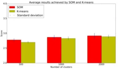
[image:6.612.332.507.650.738.2]At first, algorithms, which require predefined number of clusters in advance are evaluated: self-organizing map and k-means algorithm. Initial learning rate of SOM algorithm was set to 0.02 in all our experiments. At this test, the SOM algorithm gives better results. Moreover, the experiment showed that the number of clusters is important for the codebook quality. Table 3 shows achieved results.
Table 3: Achieved results by SOM and k-menas after ten runs (± denotes standard deviation, number in
parenthesis denotes topology of SOM.).
Number of clusters
K-means SOM
500 2.73 ± 0.04 2.78 ± 0.05
(60x50)
1000 2.83 ± 0.06 2.87 ± 0.07
(60x70)
2000 2.89 ± 0.06 2.92 ± 0.09
16 The achieved results are also illustrated in the
[image:7.612.92.290.425.658.2]Figure 4.
Figure 4: Visualization of results achieved by SOM and K-means
The next evaluated algorithm is BIRCH. This algorithm does not require to set the number of clusters in advance. The branching factor was set to 50 for all experiments and we tried multiple values of threshold, where the radius of the cluster obtained by merging a new sample and the closest cluster must be smaller than the threshold P. Results achieved by BIRCH can be seen in Figure 5 and in the Table 4. The measure of performance is the number of relevant images among top four retrieved images.
Table 4: Results achieved by BIRCH.
Threshold Number of clusters
Score
305 2193 2.747
310 1365 2.84
315 884 2.81
320 439 2.78
Figure 5: Visualization of results achieved by BIRCH.
The last evaluated algorithm is Mean-shift. This algorithm is not suited for the large amount of data due to its time complexity, so we did only one experiment. It has only one parameter which must be set in advance - the bandwidth. We set bandwidth to 360. The algorithm reached the worst score of all tested algorithms. The only advantage of this algorithm is that it is fully deterministic. The algorithm reached score 2.18 and found 1618 clusters.
DBSCAN algorithm did not work well with this dataset. We were not able to find proper parameter values and it always led to small amount of clusters. The maximal number of discovered clusters was 7 and it is not enough for Bag of Visual Words representation. The reached score was only 1.12. The problem can be caused by clusters with varying density. The performance of the evaluated algorithms is illustrated in the Figure 6.
Figure 6: The best results achieved by evaluated algorithms after ten runs.
The examples of query results are in figure 7 and 8.
[image:7.612.317.520.524.646.2] [image:7.612.103.283.549.658.2]
17
Figure 8: Example of query results. The visual codebook was created with SOM with topology (60x70) and initial learning rate 0.02. The number of clusters was set to 500.
7.2 Classification
We indorse that for this dataset is not necessary use codebooks with high amount of visual words as can be seen in [22]. The self-organizing map and the k-means had defined number of clusters to 100 whereas other algorithms do not require to set it appriori. The size of grid of self-organizing map was set to 40x50.
[image:8.612.89.299.490.571.2]The DBSCAN algorithm was evaluated for different values of parameter
U
, but it never found more than 76 clusters. The minimal amount of instances in the cluster was set to 20 and the value ofU
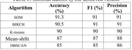
was empirically set to 41.Table 5: Summarization of the achieved results
Algorithm Accuracy
(%) F1 (%)
Precision (%)
SOM 91.3 91 91
BIRCH 90.5 91 91
K-means 90 90 90
Mean-shfit 87 87 88
DBSCAN 85 85 86
The means-shift algorithm was evaluated with bandwidth 350.94. We found this value empirically. In Figure 9 can be seen visualization of visual codebook. In Table 5 and in Figure 10 can be seen the evaluation of tested clustering algorithms.
Figure 9: Visualization of visual codebook. In the line are parts of images considered to be the same visual
word
Figure 10: Visualization of the results with evaluated algorithms. It the parentheses can be seen number of
clusters
8. DISCUSSION
Several different clustering approaches to codebook generation were presented and experimentally evaluated at image retrieval system and classification task. The best results were obtained with self-organizing map. BIRCH was slightly worse than self-organizing map in accuracy, but time complexity of BIRCH is better. The evaluation is done by classification and image retrieval.
The advantage of k-means and mean-shift is that it only needs to know one parameter in advance. BIRCH and DBSCAN need to know two parameters in advance, whereas SOM needs to set topology, learning rate and the number of iterations.
The advantage of SOM and BIRCH is that if there new images arrive, we can run some training iterations with new images, whereas other algorithms must be trained on whole dataset again.
The advantage of BIRCH, DBSCAN and mean-shift is that they can automatically set t h e number of clusters whereas k-means and SOM need this information in advance.
18 logarithmic time complexity, but it cannot find a sufficient number of clusters and it is not deterministic. BIRCH has logarithmic time complexity too and it performs well on the both dataset, furthermore it is deterministic.
DBSCAN has an ability to find any shape of the clusters so representative sample for a cluster cannot be used. According to this ability we used classification algorithm for assigning new instances to the clusters. Classification must be performed fast, because of amount of local descriptors so forests of randomized trees was used. Remaining discussed algorithms have a representative sample of the cluster, so the new instance can be assigned to the cluster with the nearest representative sample.
Our experiments have shown that the number of visual words in the codebook must be set carefully. It is not easy to say how many visual words is in given dataset, so we have to try several values. In classification experiment was 100 clusters enough, whereas in image retrieval the best performance was achieved with 2000 clusters.
9. CONCLUSION AND FUTURE WORK
This paper is focused on the empirical evaluation of different clustering approaches for visual codebook generation. Visual codebook is important part of Bag of Visual Words representation. The visual codebook is generated by clustering descriptors of local features. For clustering can be used many different algorithms which are similar in their goals, but have an algorithmically different approach.
In this paper we evaluated five different algorithms that can be used for visual codebook generation. The evaluation is done by classification and image retrieval.
The measure of performance for image retrieval experiment was number of relevant images at the top four retrieved images. In both tasks, the best results were obtained with SOM algorithm, but k-means and BIRCH were able to create good codebooks too. The measure of performance for classification task was accuracy, precision and F1 measure. The best accuracy was reached SOM algorithm, but BIRCH and k-means were just a little bit worse.
In the both experiments the worst results performed the DBSCAN algorithm. The problem of DBSCAN was to find suitable values for his parameters. DBSCAN reached the worst performance in all measured measures. On the
other hand, DBSCAN has a logarithmic time complexity.
In the future work we will investigate the weaker performance of the density based algorithms and we will evaluate proposed algorithms with different local features extraction methods.
ACKNOWLEDGEMENT
This work was partially supported by the Scientific Grant Agency of Slovakia, grant No. VG 1/0752/14.
REFRENCES:
[1] Benesova W., Kottman M. and Sidla O., “Hazardous sign detection for safety applications in traffic monitoring”, in SPIE Volume 8301, 2012
[2] Jurie, F. and Triggs, B, “Creating Efficient Codebooks for Visual Recognition.” in Proceedings of the Tenth IEEE International
Conference on Computer Vision (ICCV’05)
Volume 01, 2005, pp. 604–610
[3] Triggs B., Jurie F., “Creating Efficient Codebooks for Visual Recognition.” in
Computer Vision (ICVV), Tenth IEEE
International Conference on (Volume: 1), 2005 [4] Lowe D.G., “Object Recognition from Local
Scale-Invariant Features.” inProceedings of the International Conference on Computer Vision-Volume 2, 1999
[5] David G. Lowe., “Distinctive image features from scale-invariant keypoints.” in int. J. Comput. Vision, 2004, ISSN 0920-5691. [6] Wójtowicz A. "Rozpoznawanie obiektów na
podstawie bazy wiedzy. Aplikacja wspierajaca rozgrywanie gier miejskich na platforme Android.”, 2012
[7] Bay H., Ess A., Tuytelaars T and Gool L.V., "Speeded-up robust features (surf) ." in Comput. Vis. Image Underst., pp. 346–359
[8] Rublee E., Rabaud V., Konolige K., and Bradski G.,”Orb: An efficient alternative to sift or surf. ” in Proceedings of the 2011 International Conference on Computer Vision (ICCV), 2011, pp. 2564–2571
19 [10] Viitaniemi V., Laaksonen J., "Spatial Extensions
to Bag of Visual Words ", in Campus Information & Visitor Relations, 2009
[11] Lloyd S. P., "ªLeast Squares Quantization in PCM", º IEEE Trans. Information Theory, vol. 2, 1982, pp. 129-137
[12] Wen G., Tang Y., Wu M., Huang Z., “Scene classification based on the contextual semantic information of image", in Journal of
Theoretical and Applied Information
Technolog, Vol. 50 No.1, 2013
[13] Jurie F., Triggs B. and Moosmann F., "Fast Discriminative Visual Codebooks using Randomized Clustering Forests", in Neural Information Processing Systems (NIPS), 2007 [14] Polčicová G., Tiňo P., “Making sense of sparse
rating data in collaborative filtering via topographic organization of user preference patterns.” in Neural Networks, Elsevier, 2004,
pp. 1183–1199
[15] Törönen P., Kolehmainen M., Wong G., Castrén E., “Analysis of gene expression data using self-organizing maps.” inFEBS Letters, 1999 [16] Štefanko M., Kvasnička V., Beňušková L.,
Pospíchal J., Farkaš I., Tiňo P, and. Král’, A.,
“Úvod do teórie neurónových sietí .” Iris, 1997 [17] Zhang T., Ramakrishnan R., and Livny M.,
"BIRCH: An Efficient Data Clustering Method for Very Large Databases", inSIGMOD, 1996 [18] Ester M., Kriegel H., Sander J. and Xu X., "A
Density-Based Algorithm for Discovering Clusters in Large Spatial Databases with Noise." in Evangelos Simoudis, 1996, pp. 226– 231
[19] Fukunaga, K.; Hostetler, L., "The estimation of the gradient of a density function, with applications in pattern recognition," in Information Theory, IEEE Transactions on, vol.21, no.1, 1975, pp. 32-40
[20] Breiman L., "RANDOM FORESTS", in Machine Learning, 45(1), 2001
[21] Nistér D. and Stewénius H., "Scalable recognition with a vocabulary tree.” in IEEE Conference on Computer Vision and Pattern Recognition (CVPR), 2006, pp. 2161-2168 [22] Kinnunen T., Kamarainen J., Lensu L., and