Regularization and Adaptation for the
Approximation of Nonsmooth Solutions for
Fredgolm First Kind Integral Equations
T.I. Serezhnikova
Institute of Mathematics and Mechanics UrB RAS, Ural Federal University,Ekaterinburg, Russia
∗Corresponding Author: [email protected]
Copyright © 2014 Horizon Research Publishing All rights reserved.
Abstract
In the paper, we propose a new regulariza-tion algorithm based on the generalized Tikhonov regu-larization method.In the paper proposed technique treats problems in the form of Fredholm first kind integral equations which must be inverted.
In classical regularization functionals we propose put in the specialize summand, which allows to distribution control of points of approximate solutions.
The best additional summand one can get with using more information about solutions.
There are six model numerical results in the paper. Numerical experiments prove, that our technique does a better job of preserving functions jumps.
As result in the case of the image reconstructions problems, we obtain approximate solutions of better accuracy and images become more blur-free images.
Keywords
Image Reconstruction; Nonsmooth So-lutions; Ill-posed Problems; Tikhonov Regularization; Integral Equations; Adaptive Method1
Introduction
The field of inverse problems is of large interest due to the importance of applications to science and industry. Since most inverse problems cannot be solved analyti-cally, computational methods play a fundamental role. There are many techniques to treat inverse problems formulated in the form of Fredholm first kind integral equations which must be inverted.
Inverse problems typically involve the quantities based on indirect measurements, so that noise in the data can cause significant errors in computational results. Tech-niques known as regularization methods have been de-veloped to deal with this ill-posedness.
In the paper, we describe two new regularizing al-gorithms for numerical reconstructing nonsmooth so-lutions of the Fredholm first kind integral equations.
These two algorithms are based on generalized Tikhonov regularization with non-differentiable functionals.
The main goal of our research is to develop numerical techniques (based on Tikhonov regularization methods) which provide efficient approximations of nonsmooth so-lutions for Fredholm first kind integral equations.
The problem of the reconstruction of blurred and noisy images is a source of many interesting models.
In the problem of the reconstruction of images, objects (pre-images) are specified by two-dimensional functions. For these functions, many plane cutting lines may be kinked functions, may have points of the function dis-continue, points of function jumps. The main goal of our numerical experiments is to construct algorithms which provide better approximations of such functions.We pro-pose the special summand put in algorithms formulas. This summand allows to distribution control of points on such lines of approximate functions.
As result, we obtain approximate solutions of better accuracy and reconstructed images become more accu-rate. Of cause, the best additional summand we can get with using more information about solutions.
We use iterative technique known as the subgradient method providing efficient means of solving linear sys-tems, which are large and ill-conditioned.
In the paper, we describe numerical results and demonstrate figures for six models. We emphasize two models for the atmospheric optics deblurring problem.
One can examine numerical results and compare how our technique does a better job of preserving func-tions jumps in both one-dimensional models and two-dimensional ones.
We want to demonstrate our figures of models and to inform the scientific community about our numerical results. We do not intend to carry out any proofs in this paper. One can see that our technique allows researchers to compute image reconstructions and to get more blur-free images.
com-cialize summand. In Subsection 5.2, one can examine graphic results to compare two techniques for image de-blurring reconstructions. Section 6 contains conclusions and acknowledgements.
2
Problem Formulation
In this section we consider two regularization tech-niques for linear operator equations. LetA:U →F be a linear operator, and let U and F be linear normed spaces. Assume that the inverse operatorA−1is
discon-tinuous, then the equationAu=f is said to be ill-posed problem.
Abstract methods with full investigation convergence of two regularization algorithms for this problem pre-sented in [1–4].
Let fδ be inaccurate data to f, ||f −fδ|| ≤ δ. The
foundation of the first regularization method is given by
min{||Au−fδ||C[Π]+α||u||Hµ :u∈Hµ[Π]}, (1)
where
||u(x)||Hµ = max
x∈Π|u(x)|+x1,x2sup∈Π
|u(x1)−u(x2)|
|x1−x2|µ
, (2)
Hµ=Hµ[Π] presents the norm in the Lipschitz space
of functions, and Π is a compact set.
The foundation of the second regularization method is given by
min{||Ahu−fδ||2L2+α(||u|| 2
L2+J(u)) : u∈U
}
,
(3) here
J(u) = ∫
D
|∇u|dx, (4)
where ∇u denotes the gradient of smooth function
u, (u∈W1
1(D)), J(u) is the total variation of the
func-tionu onD.
Usually, in regularization methods the proper regular-ization parameterαwill give an approximation solution, which may be overly smooth. Our goal is to reconstruct nonsmooth solutions.
We propose to combine two process: the Tikhonov variational representations (1)–(4) and the version of the iterative technique, see [5-7]. Then, the result procedure generates a sequence{uk}by takinguk to be the
mini-mizer
uk= arg min{Φα(u) +β||u−uk−1||2 :u∈U}
≡arg min{Φα,β(u;uk−1)}, β >0, (5)
where Φ (u) is functional in (1) or in (3), ||·||denotes Hilbert norm.
In order to computeukdefined in (5), we use iterative nonlinear subgradient method
uk−1, ν+1=uk−1, ν−λk−1
vk−1, ν
||vk−1, ν||, ν = 0,1,2, ..., nk−1,
(6)
wherevk−1, ν∈∂Φα,β(uk−1, ν), Φα,βis functional in (5), and ∂Φ is an arbitary subgradient of the func-tional Φ.
Stability of process (6) is guaranteed provided that the functional in (5) is strong convex, see [3].
3
Numerical
Experiments
in
One-Dimensional Space
First of all, we tested the regularization method (1),(2),(5),(6) for the one-dimensional problem.
Consider the Fredholm first kind integral equation
Au≡ 2
∫
0
H
H2+ (x−y)2u(x)dx=f(y),
0< H≤2,0≤x, y≤2. (7)
The inverse problem associated with the model equa-tion (7) is the following. Given measurements f(y) on the earth’s surface, reconstruct the subsurface gravita-tion field u(x).The parameter H represents the depth. We are interested in reconstructions of nonsmooth so-lutions. The model functions utrue were taken to be
piecewise linear.
We selected the proper constantβ in (5) for each nu-merical experiments.
Our numerical experiments proved that it is useful to changeβ if we have changed amount of mash points; see details in [3]. The initial guess was taken to be a zero vectoru0= 0 in (5).
We used the relative iterative solution error norms to measure numerical performance in tests
∆1=||
utrue−u˜α||L2
||utrue||L2
, ∆2=||
Au˜α−f||L2
||f||L2 ,
whereutrueis the true solution of the functional
equa-tion in (7) and ˜uαrepresents the numerical
approxima-tion to utrue. One can see solution error quantities and
other details in the paper [3].
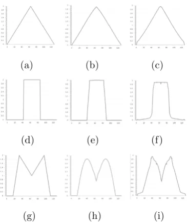
In this paper we only present nine plots of numeri-cal test results for the one-dimensional problem (7); see Figure 1.
(a) (b) (c)
(d) (e) (f)
[image:3.595.86.269.52.269.2](g) (h) (i)
Figure 1. Models and numerical solutions. (Mesh points: xi= ih, i= 0, ...,128, h = 1/n, n= 128). Plots in the first column show three true solutions. Plots in the second column represent reconstructions in the case of the numerical exactf in (7). The third column consists of reconstructionsuin the case of noisy data
f in (7).
4
Mathematicall Model for
Im-age Deblurring
We consider the follwing two-dimensional Fredgolm first kind integral equation:
Au≡ 1
∫
0 1
∫
0
K(x−ξ, y−η)u(x, y)dx, dy=f(ξ, η). (8)
In image reconstruction, the estimation ofufrom ob-servation offis referred to as the two-dimensional image deblurring problem.
In optics,uis called the light source, or object. The kernel functionK is known as the point spread function (PSF), andf is called the blurred image. The image is often recorded with a device known as a CCD camera.
We are interested in reconstructions of nonsmooth so-lutions. Using total variation, one can effectively recon-struct functions with jump discontinuities.
We construct the original method (see (3),(4) together with (5),(6)) to solve problem (8). The practical imple-mentation of this method requires the minimization of a discretized version of the functional in (8). A com-pletely discrete model may be obtained by truncating the region of integreation in (8) to be the union of the small squares h×h, h = 1./n and then applying the midpoint quadrature to (8). So, equations (3)–(6) are reduced to
min {∑
k,l h2[∑
i,j
h2K(yk−ti, yl−sj)u(ti, sj)−fk,l
]2
+α∑ i,j
h2{u2 i,j+
[(
ui,j−ui,j−1 h
)2
+ (
ui,j−ui−1,j
h
)2]1 2}}
,(9)
uk= arg min{ΦαN(u)+∑
i,j
βi,j(ui,j−uki,j−1)
2 :u∈RN}.
(10)
Here, N =n2,Φα
N(u) is functional in (9).
We use the iterative subgradient method in order to computeuk defined in (10)
uk, ν+1=uk, ν−λk
vk, ν
||vk, ν||, ν= 0,1,2, ..., nk, (11)
where vk, ν ∈ ∂Φα,β
N (uk, ν) is the functional in (10),
and ∂Φ is an arbitary subgradient of the functional Φ.
5
Adaptive Function
β
(
x, y
)
5.1
MotivationFor the one-dimensional problem, we used constant parameterβin every points for the same discrete model. It may be useful to change parameter β if we have changed amount of mash points, see details in [3].
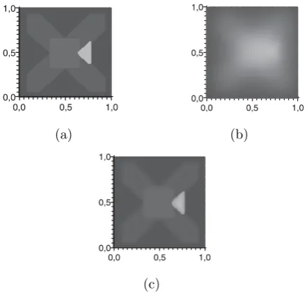
The first model for the two-dimensional problem (see Figure 2(a)) is resembling the second model, see Figure 1(d), for the one-dimensional problem. Namely, failure of the initial calculations for the model in Figure 2 mo-tivated us to change the way ofβi,j selection. Now, we
propose to use an adapted βi,j. We set
{
βi,j= 10−10 for the points,whereutrue = max{utrue}, βi,j= 0, whereutrue<max{utrue}.
(12)
If the true solution utrue is unknown, in the opinion
of the author, we can make use of the approximation ˜
uk, k= 0,1, ... .But, it is outside the scope of this paper.
5.2
Comparisons with Total Variation Regu-larization Solutions for Image Deblurring ReconstrutionsWe now compare numerical results obtained for set-ting a zero parameterβ, β≡0,and numerical results for adaptedβi,jin (10). One can see that our numerical
al-gorithm (3)–(6) with the parameterβ≡0 is a variant of the Tikhonov total variation regularization technique in two-dimensional case. In order to demonstrate the qual-itative difference between numerical results obtained for setting β ≡ 0 and for setting adapted βi,j, we present
(a) (b)
[image:4.595.63.539.54.282.2](c)
Figure 2. First model image reconstruction. (a) Plot shows the true object. (b) Plot shows blurred image. (c) Plot shows reconstrution from data (b).
[image:4.595.323.542.357.463.2]factors. Our numerical results produce visual compar-isons of these two solution techniques for two tests, see Figure 3 and Figure 5.
In order to compare the results, we present the plot of the true image diagonal and plots of the corresponding reconstruction diagonals in Figure 4.
For the solution of equation (8), the diagonal
utrue(x, x) of the true image, see Figure 3(c), is given
by
utrue(x, x) =
2.5×10⁻⁴, 0.391≤x <0.484,
0.531≤x <0.625; 0. , otherwise.
(13)
In Figure 4, we have visual comparisons of two so-lution reconstructions for blurred image in Figure 3(a). One can see that the algorithm with adaptedβi,jdoes a
better job of preserving jumps of the function (compare Figure 4(b) with Figure 4(a)).
The base configuration for the true model in Figure 5(a) is taken from [8]. In Figure 5(a) the most interesting detail is the white triangle. Figure 6 demonstrates visual comparisons of two reconstructions for this triangle. One can see in Figure 6(b), due to adaptedβi,jthe plane
triangle reconstruction is better (compare with Figure 6(a)).
Now we consider some explanation for the white tri-angle reconstruction in Figure 5(a). Let any fixed point
Alies into the white triangle and any fixed pointB lies out the triangle, so the point A is a white point, the pointB is a dark point.
In our tests, for the true solution there is the point
C, C ∈ [A, B], that every point in the interval [A, C] is a white point and every point in the interval (C, B] is a dark point.
In our tests, for the algorithm with β ≡0 the result approximate solution has some intervals as [A, B], which
(a) (b)
(c)
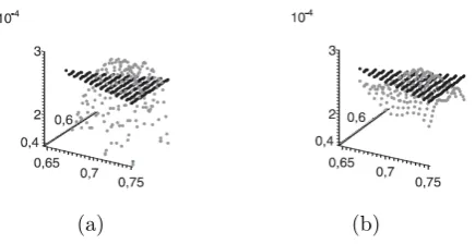
Figure 3. Second model image reconstruction. (a) Plot shows blurred image. (b) Plot shows reconstrution from data (a) for adaptedβi,j(see (12)). (c) Plot shows the true object in the
three-dimensional coordinate system.
[image:4.595.321.542.548.760.2](a) (b)
Figure 4. A plot of the true image diagonal (13) and recon-struction diagonals. (a) Plots show the true image diagonal and the reconstruction diagonal for β ≡ 0.(b) Plots show the true image diagonal and the diagonal reconstructed with the adapted
βi,jgiven by (12).
(a) (b)
(c)
(a) (b)
Figure 6. Plots demonstrate visual comparisons of two recon-structions for the image model in Figure 5 (a). (a) Plots show the true solution triangle part and the reconstruction of the triangle part forβ≡0; (b) Plots show the true solution triangle part and the reconstruction of the triangle part for adaptedβi,j.
not at all contain white points. So, some part of the triangle is ”destroyed”.
At the same time, the algorithm with adapted βi,j
”save” many ”almost white” points in the interval [A, C].
So, the visual result is quite better in the algorithm with adaptedβi,j.
Additionally, let us consider finish steps of algorithms. If algorithm withβ≡0 is finished at the iteration num-ber k (k is number of iteration that were required to satisfy the stopping criterions), then we set the approx-imate solution ˜uis equal to ˜uk, ˜u= ˜uk.
Then, for the algorithm with adapted βi,j we start
with ˜ukas the initial approximation for iterations. Note,
that due to the selection of the proper large βi,j in
points of the white triangle, we have Φα,βN (u,uk)) ≫
Φα,0N (u,uk), |∂Φα,β N (u,u
k))| ≫ 0, where Φα,β N , ∂Φ
α,β N
from (10).
We continue computations with adapted βi,j. Then,
we get ˜uk+1, which is nearer to exact solution than ˜uk:
as we see in tests, number of white points in the tri-angle for ˜uk+1 is more than number of white points in the triangle for ˜uk. So the approximation of the trian-gle configuration is more exact for the algorithm with adaptedβi,j.
6
Conclusions
In this paper we present two new regularizing al-gorithms for numerical reconstructing nonsmooth solu-tions of Fredholm first kind integral equasolu-tions. We pro-pose the specialize summand put in classical regularizing functionals containing regularization parameterα.
Proposed summand construction uses the true solu-tion or some informasolu-tion about it. We mean, for ex-ample, the information about lines consisting of points of discontinuities of the functionutrue and the
informa-tion about the max value of the funcinforma-tionutrue.In model
calculations, we used specialize summand in the form which one can see in (12) for the two-dimensional case. The more general form of this summand for the two-dimensional case may be given by
I= ∫
Q
β(x, y)[u(x, y)−uk(x, y)]2dxdy,
where
{
β(x, y) =umax, for (x, y) ∈Q, β(x, y) = 0, for (x,y)∈Π/Q,
umax= max
Π {utrue(x, y)},Π = [0,1]×[0,1],
(x, y)∈Q⇔u(x, y) =umax.
Above one can see that β(x, y) is piece-wise constant function and the function β(x, y) is depending on the function utrue. One can try to use uk(x, y) instead of utrue.
In the paper, we describe numerical experiments and demonstrate six Figures for models. Two of demon-strated tests are related to the atmospheric optics de-blurring problem.
One can see and compare in figures that our tech-nique does a better job of preserving functions jumps in both one-dimensional models and two-dimensional ones due to adapting of the function β(x, y). Comparisons of reconstructions in Figure 4 and comparisons of re-constructions in Figure 6 show that the adapted func-tionβ(x, y) ensures crucially improve of reconstructions quality for nonsmooth solutions. As result, we see in Figure 3 and Figure 5 that reconstructed images appear accurate enough images, appear more blur-free images.
There is an obvious direction of the future work. We shall try to reconstruct images which contain several complicated details. The main purpose remains to improve reconstructions of function jumps and to get more blur-free images.
Acknowledgments
The author would like to express special gratitude to Prof. V.V.Vasin, from the Institute Mathematics and Mechanics UrB RAS.
This work is supported by RFBR project no. 12-01-00106.
REFERENCES
[1] V.V. Vasin. Stable approximation of nonsmooth solu-tions to ill-posed problems, Dokl. Math. Vol.71, No.3, 419–422, 2005.
[2] V.V. Vasin. Regularization and iterative approximation for linear ill-posed problems in the space of functions of bounded variation, Proc. Steclov Inst. Math. Suppl. Vol.12, No.1, 64–77, 2002.
[3] V.V. Vasin and T.I. Serezhnikova. A regularizing algorithm for approximation of a nonsmooth solution of Fredholm integral equations of the first kind, J. VICH. TECH., Vol.15, No.2, 15–23, 2010.
[6] B. Martinet. Determination approachee d’un point fixe d’ne Applications pseudo-contrctante , C.R. Acad. Sci. Paris., Vol. 274, 163-165, 1972.