New Gradient Methods for Bandwidth Selection in Bivariate Kernel Density Estimation

(1)

New Gradient Methods for Bandwidth Selection in

Bivariate Kernel Density Estimation

Siloko, I. U.1,*_{, Ishiekwene, C. C.}2_{, Oyegue, F. O.}2

1_{Department of Mathematical Sciences, Edwin Clark University, Nigeria}

2_{Department of Mathematics, University of Benin, Nigeria}

Abstract

The bivariate kernel density estimator is fundamental in data smoothing methods especially for data exploration and visualization purposes due to its ease of graphical interpretation of results. The crucial factor which determines its performance is the bandwidth. We present new methods for bandwidth selection in bivariate kernel density estimation based on the principle of gradient method and compare the result with the biased cross-validation method. The results show that the new methods are reliable and they provide improved methods for a choice of smoothing parameter. The asymptotic mean integrated squared error is used as the measure of performance of the new methods.

Keywords

Bandwidth, Bivariate Kernel Density Estimator, Biased Cross-validation, Gradient Method, Asymptotic Mean Integration Squared Error

1. Introduction

Kernel density estimators are widely used nonparametric estimation techniques due to their simple forms and smoothness. Kernel density estimation is the construction of a probability density estimates from a given sample with few assumptions about the underlying probability density function and the kernel function. Kernel density estimation is a popular tool for visualising the distribution of data [1]. These estimates depend on a bandwidth also known as the smoothing parameter which controls the smoothness and a kernel function which plays the role of a weighting function [2]. Bandwidth selection is a key issue in kernel methods and has attracted the attention of researchers over the years. It is still an active research area in kernel density estimation. Progress has been made recently on data based

smoothing parameter selectors by some researchers [3, 4]. The importance of the bivariate kernel density estimator cannot be overemphasized because it occupies a unique position of bridging the univariate kernel density estimator and other higher dimensional kernel estimators [5]. The usefulness of the bivariate kernel density estimator is mainly in its simplicity of presentation of probability density estimates, either as surface plots or contour plots. It also helps in understanding other higher dimensional kernel estimators [2]. In bivariate kernel density estimation, 𝐱𝐱 , 𝐲𝐲 is taken to be the two random variables with a joint probability density function 𝒇𝒇(𝐱𝐱 , 𝐲𝐲). The random variables 𝐗𝐗𝒊𝒊, 𝐘𝐘𝒊𝒊, 𝒊𝒊 = 𝟏𝟏, 𝟐𝟐, … , 𝒏𝒏 are the set of

observations and 𝒏𝒏 is the sample size. The bivariate kernel density estimate of 𝒇𝒇(𝐱𝐱 ,𝐲𝐲) is of the form

𝒇𝒇�(𝐱𝐱 ,𝐲𝐲) =_{𝒏𝒏𝒉𝒉}𝟏𝟏

𝐱𝐱𝒉𝒉𝐲𝐲∑ 𝑲𝑲

𝒏𝒏

𝒊𝒊=𝟏𝟏 �𝐱𝐱−𝐗𝐗_𝒉𝒉_𝐱𝐱𝒊𝒊,𝐲𝐲−𝐘𝐘_𝒉𝒉_𝐲𝐲𝒊𝒊� (1.1)

where 𝒉𝒉𝐱𝐱> 0 and 𝒉𝒉𝐲𝐲> 0 are the smoothing

parameters in the 𝐗𝐗 and 𝐘𝐘 axes and 𝑲𝑲(𝐱𝐱 ,𝐲𝐲) is a bivariate kernel function [5, 6]. The bivariate kernel density estimator in (1.1) can be written as [7]

𝒇𝒇�(𝐱𝐱 ,𝐲𝐲) =𝟏𝟏_𝒏𝒏∑ _𝒉𝒉𝟏𝟏

𝐱𝐱𝑲𝑲

𝒏𝒏

𝒊𝒊=𝟏𝟏 �𝐱𝐱−𝐗𝐗_𝒉𝒉_𝐱𝐱𝒊𝒊�_𝒉𝒉𝟏𝟏_𝐲𝐲𝑲𝑲 �𝐲𝐲−𝐘𝐘_𝒉𝒉_𝐲𝐲𝒊𝒊� (1.2)

Bivariate bandwidth selection is a difficult problem which may be simplified by imposing constraints on 𝒉𝒉𝐱𝐱

and 𝒉𝒉𝐲𝐲. For example, 𝒉𝒉𝐱𝐱 and 𝒉𝒉𝐲𝐲 may be restricted to be

the diagonal elements of the bandwidth matrix and the advantages of imposing restrictions on 𝒉𝒉𝐱𝐱 and 𝒉𝒉𝐲𝐲 has

(2)

𝑩𝑩𝑩𝑩𝑩𝑩�𝒉𝒉𝐱𝐱, 𝒉𝒉𝐲𝐲� =_{𝟒𝟒𝝅𝝅𝒏𝒏𝒉𝒉}𝟏𝟏_𝐱𝐱_𝒉𝒉_𝐲𝐲+ _{𝟒𝟒𝒏𝒏(𝒏𝒏−𝟏𝟏)𝒉𝒉}𝟏𝟏 _𝐱𝐱_𝒉𝒉_𝐲𝐲 × ∑𝒊𝒊=𝟏𝟏𝒏𝒏 ∑ ��∆𝒋𝒋≠𝒊𝒊 𝟏𝟏𝟐𝟐+ ∆𝟐𝟐𝟐𝟐�𝟐𝟐− 𝟖𝟖�∆𝟏𝟏𝟐𝟐+ ∆𝟐𝟐𝟐𝟐� + 𝟖𝟖� 𝝓𝝓(∆𝟏𝟏)𝝓𝝓(∆𝟐𝟐) (1.3)

where ∆𝟏𝟏= �𝐱𝐱−_𝒉𝒉𝐗𝐗_𝐱𝐱𝒊𝒊�, ∆𝟐𝟐= �𝐲𝐲−_𝒉𝒉_𝐲𝐲𝐘𝐘𝒊𝒊� and 𝝓𝝓 is the standard normal density function.

This paper focuses on the methods of selecting bandwidth for bivariate kernel density estimator using the gradient methods. The rest of the paper is organized as follows: in section 2, we present the asymptotic mean integrated square error of the bivariate kernel density estimator; in section 3, we present the gradient methods while section 4 talks about numerical illustrations of results. Section 5 concludes the paper.

2. Asymptotic MISE Approximations

The estimate 𝒇𝒇�(𝐱𝐱 , 𝐲𝐲) in (1.2) is measured by the asymptotic mean integrated squared error (AMISE). A straightforward asymptotic approximation of (1.2) using the multivariate version of Taylor’s series expansion yields the integrated variance (IV) and the integrated squared bias (ISB) as

� 𝑰𝑰𝑩𝑩 =

𝑹𝑹(𝑲𝑲)𝒅𝒅

𝒏𝒏𝒉𝒉𝐱𝐱𝒉𝒉𝐲𝐲 and

𝑰𝑰𝑰𝑰𝑩𝑩 =𝟏𝟏_𝟒𝟒𝝁𝝁𝟐𝟐(𝑲𝑲)𝟐𝟐∫𝒕𝒕𝒕𝒕𝟐𝟐�∑ 𝝏𝝏

𝟐𝟐_{𝒇𝒇(𝐱𝐱,𝐲𝐲)}

𝝏𝝏𝐱𝐱𝟐𝟐_{𝝏𝝏𝐲𝐲}𝟐𝟐

𝟐𝟐

𝒋𝒋=𝟏𝟏 𝒉𝒉𝟐𝟐𝐱𝐱𝒉𝒉𝟐𝟐𝐲𝐲� 𝒅𝒅𝐱𝐱𝒅𝒅𝐲𝐲

(2.1)

where 𝑹𝑹(𝑲𝑲) is the roughness of the kernel, 𝒕𝒕𝒕𝒕 is the trace of a matrix (matrix of second partial derivatives) of 𝒇𝒇, 𝒅𝒅 is the dimension of the kernel and 𝝁𝝁𝟐𝟐(𝑲𝑲)𝟐𝟐 is the second moment of the kernel. Combining the terms in (2.1) yields an

estimate of the asymptotic mean integrated squared error and is of the form

𝑨𝑨𝑨𝑨𝑰𝑰𝑰𝑰𝑨𝑨 =_{𝒏𝒏𝒉𝒉}𝑹𝑹(𝑲𝑲)𝒅𝒅

𝐱𝐱𝒉𝒉𝐲𝐲+

𝟏𝟏

𝟒𝟒𝝁𝝁𝟐𝟐(𝐊𝐊)𝟐𝟐 ∫ 𝒕𝒕𝒕𝒕𝟐𝟐�∑

𝝏𝝏𝟐𝟐_{𝒇𝒇(𝐱𝐱,𝐲𝐲)}

𝝏𝝏𝐱𝐱𝟐𝟐𝝏𝝏𝐲𝐲𝟐𝟐 𝟐𝟐

𝒋𝒋=𝟏𝟏 𝒉𝒉𝐱𝐱𝟐𝟐𝒉𝒉𝟐𝟐𝐲𝐲� 𝒅𝒅𝐱𝐱𝒅𝒅𝐲𝐲 = 𝑹𝑹(𝑲𝑲)

𝒅𝒅

𝒏𝒏𝒉𝒉𝐱𝐱𝒉𝒉𝐲𝐲 +

𝟏𝟏

𝟒𝟒𝝁𝝁𝟐𝟐(𝐊𝐊)𝟐𝟐𝑹𝑹(𝒇𝒇″) (2.2)

where 𝑹𝑹(𝒇𝒇″_{) = � 𝒕𝒕𝒕𝒕}𝟐𝟐_��𝝏𝝏𝟐𝟐𝒇𝒇(𝐱𝐱,𝐲𝐲)

𝝏𝝏𝐱𝐱𝟐𝟐_{𝝏𝝏𝐲𝐲}𝟐𝟐 𝟐𝟐

𝒋𝒋=𝟏𝟏

𝒉𝒉𝟐𝟐𝐱𝐱𝒉𝒉𝐲𝐲𝟐𝟐� 𝒅𝒅𝐱𝐱𝒅𝒅𝐲𝐲 is the roughness of 𝒇𝒇″(𝐱𝐱 , 𝐲𝐲).

The smoothing parameter that minimizes the AMISE of (2.2) is given by

𝑯𝑯𝑨𝑨𝑨𝑨𝑰𝑰𝑰𝑰𝑨𝑨≈ � 𝒅𝒅𝑹𝑹(𝑲𝑲)

𝒅𝒅

𝝁𝝁𝟐𝟐(𝐊𝐊)𝟐𝟐𝑹𝑹(𝒇𝒇″)�

�_{𝒅𝒅+𝟒𝟒}𝟏𝟏 �

× 𝒏𝒏−�_{𝒅𝒅+𝟒𝟒}𝟏𝟏 �_(2.3)

The 𝑯𝑯𝑨𝑨𝑨𝑨𝑰𝑰𝑰𝑰𝑨𝑨yields an 𝑨𝑨𝑨𝑨𝑰𝑰𝑰𝑰𝑨𝑨 = 𝑶𝑶 �𝒏𝒏−�

𝟒𝟒

𝒅𝒅+𝟒𝟒�� and the bandwidths are of order 𝒏𝒏−𝟏𝟏 (𝒅𝒅+𝟒𝟒)⁄ . The problem with (2.3) is

that it has a bias term which depends on 𝑹𝑹(𝒇𝒇″₎_{and cannot be evaluated if the true density function}_𝒇𝒇_{is not known.}

Several suggestions have been made and one of the simplest solutions to this problem is to obtain the value of

𝑹𝑹(𝒇𝒇″₎_{from the normal distribution for unimodal data but for data that is multimodal (which is kernel density estimations’}

expectation), it behaves poorly in performance and in that situation, it serves as an initial point for other iterative methods [11, 12].

3. The Gradient Method

Gradient methods are iterative methods of optimizing functions that are at least twice continuously differentiable [13]. Gradient methods involve generating successive points in the direction of the gradient function with the desire to obtain the stationary points [14]. The gradient of a function 𝒇𝒇(𝐱𝐱) denoted by 𝛁𝛁𝒇𝒇(𝐱𝐱) is given by

𝛁𝛁𝒇𝒇(𝐱𝐱) = �_{𝝏𝝏𝐱𝐱}𝝏𝝏𝒇𝒇

𝟏𝟏 ,

𝝏𝝏𝒇𝒇 𝝏𝝏𝐱𝐱𝟐𝟐 , … ,

𝝏𝝏𝒇𝒇 𝝏𝝏𝐱𝐱𝒏𝒏�

𝑻𝑻

(3.1) Gradient methods are iterative techniques with the elements of the gradient being nonlinear and a positive scalar (stepsize) that determines the distance between the current point and the previous point [13]. Generally, the gradient method requires higher derivatives of the function to be approximated. In this work, we modify the gradient methods of Barzilai and Borwein and the relaxed steepest descent method of Raydan and Svaiter [15, 16].

In the application of the gradient methods, we replace the unknown quantity 𝑹𝑹(𝒇𝒇″₎_{in (2.3) by a suitable kernel based}

estimate denoted by 𝑹𝑹��𝒇𝒇(𝐱𝐱)�, i.e. 𝑹𝑹(𝒇𝒇″_{) = 𝑹𝑹��𝒇𝒇(𝐱𝐱)�}_{. The kernel function used is the standard normal kernel that}

produces smooth density estimates and simplifies the mathematical computations needed. In the case of the standard normal kernel, successive smoothing parameters will be obtained from the approximation given by

𝑯𝑯𝑨𝑨𝑨𝑨𝑰𝑰𝑰𝑰𝑨𝑨≈ �� 𝒅𝒅𝑹𝑹(𝑲𝑲)

𝒅𝒅

𝝁𝝁𝟐𝟐(𝐊𝐊)𝟐𝟐×𝑹𝑹��𝒇𝒇(𝐱𝐱)��

𝟏𝟏 (𝒅𝒅+𝟒𝟒)⁄

(3)

Since all gradient methods are iterative methods and they require the choice of a starting value say 𝐗𝐗𝐨𝐨 we apply

a kernel based estimate as an initial point for the iteration process and is of the form

𝐗𝐗𝐨𝐨= � 𝑹𝑹(𝑲𝑲)

𝒅𝒅

𝝁𝝁𝟐𝟐(𝐊𝐊)𝟐𝟐𝝈𝝈𝒋𝒋�

�_{𝒅𝒅+𝟒𝟒}𝟏𝟏 �

× 𝒏𝒏−�_{𝒅𝒅+𝟒𝟒}𝟏𝟏 �_,_(3.3)

where 𝝈𝝈𝒋𝒋 is the standard deviation of the 𝒋𝒋𝒕𝒕𝒉𝒉 variate.

3.1. The Barzilai and Borwein Gradient Method This method solves the problems associated with the classical gradient method with their novel approach of the stepsize selection. It requires lesser computations and the rate of convergence is also accelerated, though with the same search direction as the classical gradient method but with better performance [17]. The method is used for obtaining large sparse linear system of equations from the solution of partial differential equations and also applies in optimization theory due to its ease of computation and implementation [18, 19]. The Barzilai and Borwein gradient method is of the form

𝐗𝐗𝐭𝐭+𝟏𝟏 = 𝐗𝐗𝐭𝐭 + 𝐒𝐒𝐭𝐭 , 𝐭𝐭 = 𝟎𝟎, 𝟏𝟏, 𝟐𝟐, …, (3.4)

where 𝐒𝐒𝐭𝐭 = −_𝛌𝛌𝟏𝟏_𝐭𝐭and 𝛌𝛌𝐭𝐭is the stepsize. The value of the

stepsize can be obtained from (3.5) as

𝛌𝛌𝐭𝐭= 𝒈𝒈𝐭𝐭

𝐓𝐓_𝒈𝒈_𝐭𝐭

𝒈𝒈𝐭𝐭𝐓𝐓𝐀𝐀 𝒈𝒈𝐭𝐭, 𝐭𝐭 = 𝟎𝟎, 𝟏𝟏, 𝟐𝟐, …, (3.5)

where 𝒈𝒈𝐭𝐭= 𝛁𝛁𝒇𝒇(𝐗𝐗𝐭𝐭 ), 𝐀𝐀 is the Hessian matrix of 𝒇𝒇

evaluated at 𝐗𝐗𝐭𝐭 and 𝐀𝐀 must be symmetric. The value of

the kernel based estimate 𝑹𝑹��𝒇𝒇(𝐱𝐱)� must be positive, i.e. 𝑹𝑹��𝒇𝒇(𝐱𝐱)� > 0 because the smoothing parameter must be positive. The estimate 𝑹𝑹��𝒇𝒇(𝐱𝐱)� = 𝐗𝐗𝐭𝐭+𝟏𝟏 when

substituted into (3.2) will give the smoothing parameter that minimizes the AMISE. In all the gradient methods considered, the modifications were in the method of obtaining the initial point of the iteration which is kernel based and the introduction of the third step that will be used to obtain the required solution.

ALGORITHM 1 (The Modify Barzilai and Borwein Method).

STEP1. Compute 𝐗𝐗𝐨𝐨= �� 𝑹𝑹(𝑲𝑲)

𝒅𝒅

�_{𝒅𝒅+𝟒𝟒}𝟏𝟏 �

× 𝒏𝒏−�𝒅𝒅+𝟒𝟒𝟏𝟏 ��,

where 𝛔𝛔𝒋𝒋 is the standard deviation of the 𝒋𝒋𝐭𝐭𝐭𝐭 variate

for 𝒋𝒋 = 𝟏𝟏,𝟐𝟐, 𝒏𝒏 is the sample size and 𝒅𝒅 is the dimension of the kernel.

STEP2. For 𝒕𝒕 = 𝟎𝟎, 𝟏𝟏, 𝟐𝟐, …,

(a) Compute the vector 𝒈𝒈𝐭𝐭= 𝛁𝛁𝒇𝒇(𝐗𝐗𝐭𝐭 ).

(b) Compute the step size 𝛌𝛌𝐭𝐭= 𝒈𝒈𝐭𝐭

𝐓𝐓_𝒈𝒈_𝐭𝐭

𝒈𝒈𝐭𝐭𝐓𝐓𝐀𝐀 𝒈𝒈𝐭𝐭.

(c) Set 𝐒𝐒𝐭𝐭 = −_𝛌𝛌𝟏𝟏_𝐭𝐭.

(d) Update 𝐗𝐗𝐭𝐭+𝟏𝟏= 𝐗𝐗𝐭𝐭+ 𝐒𝐒𝐭𝐭 .

STEP3. Employ 𝑹𝑹��𝒇𝒇(𝐱𝐱)� = 𝐗𝐗𝐭𝐭+𝟏𝟏 to compute the

smoothing parameter using (3.2) above.

STEP4. Test a criterion for stopping the iterations. If the test is satisfied, then stop. Otherwise, consider 𝐭𝐭 = 𝐭𝐭 + 𝟏𝟏

and continue with step 2 by updating the step size,

𝛌𝛌𝐭𝐭+𝟏𝟏= 𝒈𝒈𝐭𝐭+𝟏𝟏

𝐓𝐓 _𝒈𝒈_{𝐭𝐭+𝟏𝟏}

𝒈𝒈𝐭𝐭+𝟏𝟏𝐓𝐓 𝐀𝐀 𝒈𝒈𝐭𝐭+𝟏𝟏, where 𝒈𝒈𝐭𝐭+𝟏𝟏 = 𝛁𝛁𝒇𝒇(𝐗𝐗𝐭𝐭+𝟏𝟏).

3.2. The Relaxed Steepest Descent Method

Another modification of the steepest descent method was made by Raydan and Svaiter [16] and they concluded that the poor performance of the method is a function of the stepsize and not the search direction. In solving the problem of the stepsize’s selection, they introduced a scalar called the relaxation parameter 𝜽𝜽 which lies between 0 and 2 into the classical steepest method. The classical steepest descent method is of the form

𝐗𝐗𝐭𝐭+𝟏𝟏 = 𝐗𝐗𝐭𝐭 – 𝛌𝛌𝐭𝐭𝒈𝒈𝐭𝐭 , 𝐭𝐭 = 𝟎𝟎, 𝟏𝟏, 𝟐𝟐, …, (3.6)

where 𝒈𝒈𝐭𝐭= 𝛁𝛁𝒇𝒇(𝐗𝐗𝐭𝐭 ). The introduction of the relaxation

parameter 𝜽𝜽 which is a random scalar on the interval [𝟎𝟎 , 𝟐𝟐], resulted in the modified steepest descent method which is of the form

𝐗𝐗𝐭𝐭+𝟏𝟏 = 𝐗𝐗𝐭𝐭 – 𝜽𝜽𝛌𝛌𝐭𝐭𝒈𝒈𝐭𝐭 , 𝐭𝐭 = 𝟎𝟎, 𝟏𝟏, 𝟐𝟐, …, (3.7)

where 𝛌𝛌𝐭𝐭= 𝒈𝒈𝐭𝐭 𝐓𝐓_𝒈𝒈

𝐭𝐭

𝒈𝒈𝐭𝐭𝐓𝐓𝐀𝐀 𝒈𝒈𝐭𝐭.

Multiplying the stepsize by the relaxation parameter resulted in the improvement of the method by accelerating its rate of convergence when applied to numerical problems [20]. It should be noted that when 𝜽𝜽 = 𝟏𝟏, the classical steepest descent method will be obtained and so 𝜽𝜽 ≠ 𝟏𝟏.

ALGORITHM 2 (The Modify Relaxation Method of Raydan and Svaiter).

STEP1. Compute 𝐗𝐗𝐨𝐨 = �� 𝑹𝑹(𝑲𝑲)

𝒅𝒅

�_{𝒅𝒅+𝟒𝟒}𝟏𝟏 �

× 𝒏𝒏−�𝒅𝒅+𝟒𝟒𝟏𝟏 ��,

where 𝛔𝛔𝒋𝒋 is the standard deviation of the 𝒋𝒋𝐭𝐭𝐭𝐭 variate

for 𝒋𝒋 = 𝟏𝟏,𝟐𝟐, 𝒏𝒏 is the sample size and 𝒅𝒅 is the dimension of the kernel.

STEP2. For 𝒕𝒕 = 𝟎𝟎, 𝟏𝟏, 𝟐𝟐, …,

(a) Compute the gradient vector 𝒈𝒈𝐭𝐭= 𝛁𝛁𝒇𝒇(𝐗𝐗𝐭𝐭 ) .

(b) Compute the step size 𝛌𝛌𝐭𝐭= 𝒈𝒈𝐭𝐭

𝐓𝐓_𝒈𝒈 𝐭𝐭

𝒈𝒈𝐭𝐭𝐓𝐓𝐀𝐀 𝒈𝒈𝐭𝐭 .

(c) Update 𝐗𝐗𝐭𝐭+𝟏𝟏 = 𝐗𝐗𝐭𝐭− 𝜽𝜽𝛌𝛌𝐭𝐭𝒈𝒈𝐭𝐭 .

STEP3. Employ 𝑹𝑹��𝒇𝒇(𝐱𝐱)� = 𝐗𝐗𝐭𝐭+𝟏𝟏 to compute the

smoothing parameter using (3.2) above.

STEP4. Test a criterion for stopping the iterations. If the test is satisfied, then stop. Otherwise, consider 𝐭𝐭 = 𝐭𝐭 + 𝟏𝟏

and continue with step 2 by updating the step size,

𝛌𝛌𝐭𝐭+𝟏𝟏= 𝒈𝒈𝐭𝐭+𝟏𝟏

𝐓𝐓 _𝒈𝒈_{𝐭𝐭+𝟏𝟏}

𝒈𝒈𝐭𝐭+𝟏𝟏𝐓𝐓 𝐀𝐀 𝒈𝒈𝐭𝐭+𝟏𝟏, where 𝒈𝒈𝐭𝐭+𝟏𝟏 = 𝛁𝛁𝒇𝒇(𝐗𝐗𝐭𝐭+𝟏𝟏).

(4)

relaxation parameter is chosen as 𝜽𝜽 =𝟏𝟏_𝒏𝒏because of the role of the sample size in the choice of smoothing parameter. Generally, it is known that the smoothing parameter depends very strongly on the sample size such that as the sample size increases, the smoothing parameter tends to be reduced [21]. The stopping criterion is‖𝐗𝐗𝐭𝐭+𝟏𝟏 − 𝐗𝐗t ‖ < 𝜺𝜺

with 𝛆𝛆 = 10−5_where_𝛆𝛆_{is the tolerance level. The results}

of the modify methods shall be compared with the biased cross-validation method.

4. Results and Discussion

In order to illustrate the efficiency of these methods, we compare their performances with the biased cross-validation method using the asymptotic mean integrated squared error (AMISE) as the error criterion function. The results are presented by comparing the gradient methods (Modify Barzilai and Borwein (MBB) and the Modify Relaxed Steepest Descent(MRSD)) with the Biased Cross-Validation (BCV)) for the bivariate kernel density estimator and using the asymptotic mean integrated squared error (AMISE) as the error criterion function for measuring their performance. As generally known, one method is better than the other when it gives a smaller value of the AMISE [12]. The comparison also involves the kernel estimates (graphs) of the methods considered since kernel density estimation has direct applications on data analysis such as exploratory data analysis and data visualisation [1, 2, 6].

Two sets of data were used to illustrate the results of the methods, showing in a tabular form the smoothing parameter, the Asymptotic Integrated Variance (AIV), the Asymptotic Integrated Squared Bias (AISB) and the Asymptotic Mean Integrated Squared Error (AMISE) using the bivariate standard normal kernel. An important point to note from the Tables below is that in terms of performance, the gradient methods resulted in a smaller

value of the AMISE.

One very important and notable step to be taken when examining bivariate data set is to consider the Scatterplot of the data. But as it has been in most cases, while kernel density estimate will reveal or highlight important features, Scatterplot cannot play this vital role [2]. Scatterplots have been regarded as the most frequently used tools for graphically displaying bivariate data sets but with the serious disadvantage that the eye is only drawn to the peripheries of the data cloud, while structures in the main body of the data will be hidden by the high density of the points [22]. In kernel density estimates, these disadvantages of the Scatterplots are removed because they have an advantage in the presentation of information regarding the distribution of the data set. As noted from the Scatterplots of the data sets considered, the modes are not apparent from the Scatterplot vas in the kernel density estimates and this exemplify the usefulness of the bivariate kernel density estimates for highlighting structure.

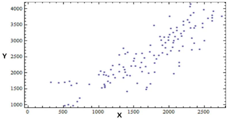
[image:4.595.100.498.538.745.2]

The first data set examined is the Volcanic Crater data of Bunyaruguru Volcanic Field in Western Uganda [23]. It involves the Locations of Centers of Craters of 120 volcanoes in two variables in which variable X represents the first center while variable Y represents the second center. Figure 1 shows the Scatterplot of the Crater data and the Scatterplot clearly show a strong relationship between the variables with correlation coefficient 𝝆𝝆 = 𝟎𝟎. 𝟖𝟖𝟏𝟏𝟒𝟒𝟖𝟖𝟖𝟖𝟖𝟖. It is evident that the two Locations of the Centers of Craters are highly positively correlated. A significant feature of this data set that is very noticeable from the kernel density estimates (graphs) is the bimodality of the data but this is hidden as presented by the Scatterplot. We standardized the data in order to obtain equal variances in each dimension because in most multivariate statistical analysis, the data should be standardized in order to make sure that the difference among the ranges of variables will disappear [2, 10, 24, 25]. Figures 2, 3, and 4 below show the kernel estimates of the Crater data.

(5)

Figure 2. Kernel Estimate of the Crater Data using BCV Smoothing Parameter

Figure 3. Kernel Estimate of the Crater Data using MBB Smoothing Parameter.

Figure 4. Kernel Estimate of the Crater Data using MRSD Smoothing Parameter

[image:5.595.111.496.79.227.2]

The biased cross-validation method yields smoothing parameter that produces an estimate with the bimodality being clearly present as shown in Figure 2. The gradient methods also yield smoothing parameter values that retain the bimodality of the data as shown in Figure 3 and Figure 4 respectively. The table below shows the bandwidths, the asymptotic integrated variance (AIV), the asymptotic integrated squared biased (AISB) and the asymptotic mean integrated squared error (AMISE) of the methods considered.

Table 1. Bandwidths, AIV, AISB and AMISE for the Crater Data

Methods. 𝒉𝒉𝐱𝐱 𝒉𝒉𝐲𝐲 𝑨𝑨𝑰𝑰𝑩𝑩 𝑨𝑨𝑰𝑰𝑰𝑰𝑩𝑩 𝑨𝑨𝑨𝑨𝑰𝑰𝑰𝑰𝑨𝑨

BCV 0.45042 0.30224 0.00487124 0.00066901 0.00554025

MBB 0.48675 0.48268 0.00282256 0.00148993 0.00431249

[image:5.595.102.501.259.401.2] [image:5.595.97.499.438.582.2] [image:5.595.91.498.689.749.2]

(6)

From Table 1 above, it is obvious that in terms of performance, the biased cross-validation method produced the largest AMISE value. The gradient methods yield a smoothing parameter with smaller AMISE value as shown in Table 1.

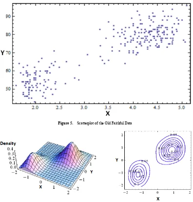
The second data set examined is the waiting time between eruptions and the duration of the eruption for the Old Faithful Geyser in Yellowstone National Park, Wyoming, USA [26]. The data set is made up of 272 observations on two variables in which variable X represents the duration of the eruption while variable Y represents the waiting time between eruptions. One very important point to note from the bivariate kernel estimates of this data is that the data set is bimodal and this provides very strong evidence in favour of eruption times and the time interval until the next eruption exhibiting a bimodal

distribution [2]. The bivariate kernel density estimates are bimodal and it is evident that the time interval until the next eruption is highly positively correlated with the duration of the eruption. The Scatterplot of the Old Faithful data is shown in Figure 5 while Figures 6, 7 and 8 are the bivariate kernel estimates of the data for the methods considered. The Scatterplot show a strong relationship between the variables with correlation coefficient 𝝆𝝆 = 𝟎𝟎. 𝟖𝟖𝟎𝟎𝟎𝟎𝟖𝟖𝟗𝟗. The data is also standardized to obtain equal variances in each dimension [24, 25].

[image:6.595.102.498.285.699.2]

Table 2 below shows the smoothing parameters, the asymptotic integrated variance (AIV), the asymptotic integrated squared bias (AISB) and the asymptotic mean integrated squared error (AMISE) of the methods considered.

Figure 5. Scatterplot of the Old Faithful Data

(7)

[image:7.595.104.500.78.222.2]

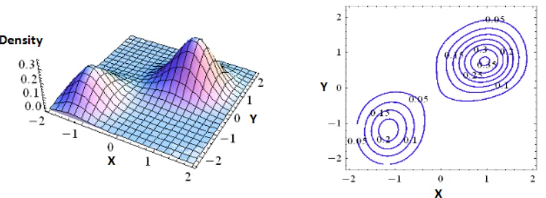
Figure 7. Kernel Estimate of the Old Faithful Data using MBB Smoothing Parameter

[image:7.595.106.498.255.397.2]

Figure 8. Kernel Estimate of the Old Faithful Data using MRSD Smoothing Parameter

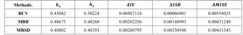
Table 2. Bandwidths, AIV, AISB and AMISE for the Old Faithful Data

Methods. 𝒉𝒉𝐱𝐱 𝒉𝒉𝐲𝐲 𝑨𝑨𝑰𝑰𝑩𝑩 𝑨𝑨𝑰𝑰𝑰𝑰𝑩𝑩 𝑨𝑨𝑨𝑨𝑰𝑰𝑰𝑰𝑨𝑨

BCV 0.29382 0.39688 0.00250897 0.00040169 0.00291066

MBB 0.36263 0.38846 0.00207688 0.00048786 0.00256474

MRSD 0.36364 0.38955 0.00206532 0.00049335 0.00255867

Table 2 shows the performances of the biased cross-validation method and the gradient methods and from the results, the biased cross-validation method yielded larger AMISE value. Again the gradient methods yield a smoothing parameter with the smaller AMISE values as presented in Table 2.

5. Conclusions

The methods presented are compared with the biased cross-validation method because they are based on a suitable estimate of the asymptotic mean integrated squared error (AMISE). The results presented show that the new methods are reliable and they provide improved methods for a choice of smoothing parameter. An advantage of the gradient methods is that they can be easily computed provided the function 𝒇𝒇 is at least twice differentiable.

As for the bivariate case that sits between the univariate

and higher dimensional kernel, and that 𝑲𝑲 is a standard normal product kernel, the gradient methods based on their performance is at least as competitive as the existing biased cross-validation.

REFERENCES

[1] Simonoff, J. S. Smoothing Methods in Statistics.

Springer-Verlag, New York, 1996.

[2] Silverman, B. W. Density Estimation for Statistics and Data

Analysis. Chapman and Hall, London, 1986.

[3] Chacón, J. E. and Duong, T. Data-Driven Density Derivative

Estimation, with Applications to Nonparametric Clustering and Bump Hunting. Electronic Journal Statistics, 7, 499–532 2013.

[4] Jiang, M. and Provost, S. B. A Hybrid Bandwidth Selection

[image:7.595.94.499.438.499.2]

(8)

Statistical Computation and Simulation, 84(3), 614–627, 2014.

[5] Duong, T. and Hazelton, M. L. Plug-In Bandwidth Matrices

for Bivariate Kernel Density Estimation. Nonparametric Statistics, 15(1), 17–30, 2003.

[6] Scott, D.W. Multivariate Density Estimation. Theory,

Practice and Visualisation. Wiley, New York, 1992.

[7] Zhange, X., Wu, X., Pitt, D. And Liu, Q. A Bayesian

Approach to Parameter Estimation for Kernel Density Estimation via Transformation. Annals of Actuarial Science, 5(2), 181–193, 2011.

[8] Wand, M. P. and Jones, M. C. Comparison of Smoothing

Parameterizations in Bivariate Kernel Density Estimation. Journal of the American Statistical Association, 88, 520–528, 1993.

[9] Scott, D. W. and Terrell, G. R. Biased and Unbiased

Cross-Validation in Density Estimation. Journal of the American Statistical Association, 82, 1131–1146, 1987. [10] Sain, R. S., Baggerly, A. K. and Scott, D. W.

Cross-Validation of Multivariate Densities. Journal of American Statistical Association, 89, 807–817, 1994. [11] Zhange, X., King, M. L. and Hyndman, R. J. A Bayesian

Approach to Bandwidth Selection for Multivariate Kernel Density Estimation. Computational Statistics and Data Analysis, 50, 3009–3031, 2006.

[12] Jarnicka, J. Multivariate Kernel Density Estimation with a Parametric Support. Opuscula Mathematica, 29(1), 41–45, 2009.

[13] Hansen, B. E. Econometrics. University of Wisconsin, Spring, 2013.

[14] Cameron. A. C. and Trivedi, P. K. Micro-econometrics Methods and Applications. Cambridge University Press, New York, USA, 2005.

[15] Barzilai, J. and Borwein, J. M. Two Point Step size Gradient

Method. IMA Journal of Numerical Analysis, 8(1), 141–148, 1988.

[16] Raydan, M and Svaiter, B. F. Relaxed Steepest Descent and Cauchy-Barzilai-Borwein Method. International Journal of Computational Optimization and Applications, 21(2), 155– 167, 2002.

[17] Raydan, M. Convergence Properties of the Barzilai and Borwein Gradient Method. A Thesis Submitted in Partial Fulfillment of the Requirements for the Degree, Doctor of Philosophy, Rice University, Houston, Texas, 1991. [18] Farid, M., Leong, W. J. and Hassan M. A. A New Two-Step

Gradient-Type Method for Large-Scale Unconstrained Optimization. Computers and Mathematics with Applications, 59, 3301–3307, 2012.

[19] Dai, Y. H. A New Analysis on the Barzilai-Borwein Gradient Method. JORC, 1, 187–198, 2013.

[20] Battaglia, J. P. The Eigenstep Method (An Iterative Method for Unconstrained Quadratic Optimization). American Journal of Operational Research, 2013, 3(2), 57–64 [21] Zambom, A. Z. and Dias, R. A Review of Kernel Density

Estimation with Applications to Econometrics. Universidade Estadual de Campinas, 2012.

[22] Wand, M. P. and Jones, M. C. Kernel Smoothing. Chapman and Hall, London, 1995.

[23] Bailey, T. C. and Gatrell, A. C. Interactive spatial data analysis. Longman, Harlow, 1995.

[24] Cula, S. G and Toktamis, O. Estimation of Multivariate Probability Density Function with Kernel Functions. Journal of the Turkish Statistical Association, 3(2), 29–39, 2000. [25] Sain, R. S. Multivariate Locally Adaptive Density

Estimation. Computational Statistics and Data Analysis, 39, 165–186, 2002.