comment
reviews
reports
deposited research
interactions
information
refereed research
Towards reconstruction of gene networks from expression data by
supervised learning
Lev A Soinov*, Maria A Krestyaninova
†
and Alvis Brazma*
Addresses: *Microarray Informatics Group and †Sequence Database Group, European Bioinformatics Institute, Wellcome Trust Genome
Campus, Hinxton, Cambridge CB10 1SD, UK.
Correspondence: Lev A Soinov. E-mail: [email protected]
Abstract
Background: Microarray experiments are generating datasets that can help in reconstructing gene networks. One of the most important problems in network reconstruction is finding, for each gene in the network, which genes can affect it and how. We use a supervised learning approach to address this question by building decision-tree-related classifiers, which predict gene expression from the expression data of other genes.
Results: We present algorithms that work for continuous expression levels and do not require a priori discretization. We apply our method to publicly available data for the budding yeast cell cycle. The obtained classifiers can be presented as simple rules defining gene interrelations. In most cases the extracted rules confirm the existing knowledge about cell-cycle gene expression, while hitherto unknown relationships can be treated as new hypotheses.
Conclusions: All the relations between the considered genes are consistent with the facts reported in the literature. This indicates that the approach presented here is valid and that the resulting rules can be used as elements for building and explaining gene networks.
Published: 6 January 2003 GenomeBiology2003, 4:R6
The electronic version of this article is the complete one and can be found online at http://genomebiology.com/2003/4/1/R6
Received: 21 June 2002 Revised: 7 October 2002 Accepted: 18 November 2002
Background
Reconstructing and modeling gene-expression networks is one of the most challenging problems of functional genomics. Large-scale monitoring of gene expression is con-sidered to be one of the most promising techniques for reconstructing gene regulatory circuits [1]. There are differ-ent approaches to describing gene networks, for example, Boolean models, models based on differential equations, and Bayesian networks, among others, but most share a common element - the expression of each gene in the network depends on the expression of some other genes [2-7]. To reconstruct such a network we have to answer two questions for each gene in the network: which genes affect it, and how
they affect it, for example, positively, negatively or in a more complex way.
play such a role in Bayesian networks, while Boolean func-tions do so in Boolean nets [5,8].
Here we describe a different approach for reconstructing ele-ments of gene networks based on predicting the expression (or changes in the expression) of a given gene from the expression (or changes in the expression) of other genes. We present our prediction results in the form of so-called classi-fiers - decision trees and decision rules. Our supervised clas-sification approach has a number of advantages. First, it allows one to identify genes affecting the target gene directly from the classifier; second, we do not have to assume any arbitrary discretization thresholds; third, each data sample is treated as an example, and classification algorithms are constructed in a way to learn from these examples (nor-mally, the more examples the higher the accuracy, usually) and finally, classifiers given in the form of decision trees or decision rules are easy to interpret.
In our model we assume that the transcription machinery of a gene can be in a finite number of different states depend-ing on the abundance of the other genes’ products, and that the expression of the gene is determined by its state. For simplicity, we consider the classifiers constructed to discrim-inate only between two states, ‘expressed more than average’ and ‘expressed less than average’, although the model can be generalized to any number of states in a straightforward manner. At the same time, there is no single threshold for absence/presence of gene products - the same gene product may affect the state of different genes at different thresholds. For instance, a particular level of a given gene product may be sufficient to switch on the expression of one gene, but may have to be raised to switch on the expression of a differ-ent gene. Our results show that this is indeed the case in real gene networks. In this way, our approach is rather different from the Boolean networks and, in fact, from any approach that depends on a prioridiscretization of expression data.
Despite rather different formulations, there is a minor simi-larity between the supervised classification and gene-expres-sion data clustering, which helps to illustrate our approach. If we know that a geneg belongs to a cluster of genes that share similar expression profiles, then, given a new sample, the behavior of the geneg can be predicted on the basis of the behavior of other genes in the cluster. Such a clustering approach can produce only ‘symmetric’ rules: for example, gene gcorrelates (or anticorrelates) with gene h. The classifi-cation rules that we derive are often more complex and can involve more than two genes, for example, gene g is expressed only if gene h1 is expressed and h2 is not expressed. It is important that our classifiers are not black boxes - they consist of sets of simple rules that can be used as elements for building and explaining gene networks, and be examined for their biological meaning. For each gene in the network we know which genes affect it, as well as a precise description of how they affect the state of the predicted gene.
We applied our methodology to the microarray datasets of Spellman and Cho for the budding yeast (Saccharomyces cerevisiae) cell cycle [9,10]. As an example, we considered a set of well-described genes, which encode proteins important for cell-cycle regulation. All extracted relations were examined with respect to the known roles of the selected genes in the cell cycle and in most cases the rules confirmed the a priori
knowledge, which indicates the validity of our approach.
Results
Definitions
Our starting point is a gene-expression data matrix, X, where each row represents a gene and each column represents a sample. Each element, xij, of Xindicates the expression level of a gene iin a sample jand is called a gene-expression value. The exact meaning of expression values may be different for different matrices, representing absolute or comparative measurements [11]. Here we use gene-expression log ratios obtained from comparisons of gene expression in a sample versus control, although, in fact, any consistent way of mea-suring gene expression can be used [12].
As already mentioned, we assume that the transcription machinery of a gene can be in a finite number of different states. Various definitions and biological interpretations of the ‘state’ are possible. For example, one can use states ‘expressed’/‘not expressed’ [8] or ‘upregulated’/‘downregu-lated’ [9]. The flexibility of the approach is that we can exploit different interpretations of states. Here we distin-guish between two different states ‘expressed more than average’/‘expressed less than average’. More precisely, we define the state, sij, of a gene iunder condition jas follows
sij =
冦
+1, ifxij> —xi, if—xiis the average expression level of ith gene,
-1, otherwise
Given a gene g, we predict its state from expression mea-surements of other genes. The geneg is called the predicted gene, while the genes on which we make the prediction are called the explaining genes. Note that the concept of state is used here only for predicted genes, while the expression values are used for explaining genes.
We will use the notation ‘simultaneous’ for the events covered by the first problem and ‘time delay’ for the second. The third problem describes events, which may or may not be sepa-rated in time and we use the notation ‘changes’ for them.
The functions determining states of predicted genes from data are called classifiers, while algorithms building such classifiers on the basis of data with known states are called inducers or induction algorithms. Each expression profile (the column of the expression matrix X) with a known state of a predicted gene is called an example or an instance. The set of examples used for classifier creation is the training set. If a subset of the examples is separated from the training set and is used for estimation of classification accuracy, it is called a test set.
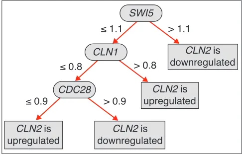
In this study we use two types of classifiers: decision trees and decision rules. A decision tree is a rooted tree in which non-leaf nodes are labeled with explaining genes, the arcs from non-leaf nodes are labeled with possible characteristics of explaining genes, and the leaves of the tree are labeled with the states of the predicted gene. An example of the deci-sion tree for classification of the yeast gene CLN2is shown in Figure 1. Each pass from the root node to a leaf node in the tree presents a rule that defines a state of the predicted gene via expression levels of explaining genes. It follows that every decision tree is equivalent to a list of decision rules (see the next section for details).
To make the verification of the classification results more straightforward we introduce a representation of classifiers in the form of simple rules. The following language for rules is used: ‘+A’ means that gene A is ‘upregulated’; ‘-A’ that gene A is ‘downregulated’, ‘<==>’ is used for simultaneous events, ‘==>’ is used to distinguish between events that are divided in time. For instance, +A+B<==>-Cmeans that Cis
‘downregulated’ when Aand Bare ‘upregulated’; +B==>+A
means that A is ‘upregulated’ if B was ‘upregulated’ (for example, in the previous time point for the time series); 앖A앗B<==>앗Cmeans that positive change in the expression level of A along with simultaneous negative change in expression of Bcoincides with simultaneous negative change of C expression; 앖B==>앗A means that positive change in expression level of Bprecedes negative change of A expres-sion. This method of representation allows the decomposi-tion of decision trees of complex structure into simple and compactly presented relations, which can be independently compared to the existing knowledge. We carried out litera-ture searches through PubMed [13] and the Yeast Protein Database (YPD) [14] to find the biological relevance of the extracted rules (see the following sections). For more precise definitions and formulations of the three problems see Materials and methods.
Classification rules
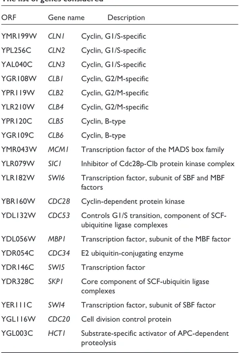
All major transitions in the budding yeast cell cycle are reg-ulated by cyclins via associated cyclin-dependent kinase (CDK) activity. To test our approach we chose a small group of yeast genes. These are the cyclin genes CLN1-3 and
CLB1-6, and CDC28, MBP1, CDC53, CDC34, SKP1, SWI4-6,
HCT1, CDC20, SIC1, and MCM1, which are involved in cell-cycle regulation and whose interactions are well described. The same set of genes (with the addition of BCK2and the exclusion of CLB3, CLB4) was used by Chen et al. [15], who presented a mathematical model of the cell-cycle events. As no reliable data were found for CLB3and BCK2 in the cdc15
dataset, we did not include them in our study (Table 1). Con-sideration of such genes made it possible to compare our results with existing knowledge.
We carried out two computational experiments and compared their results. In the first experiment we considered eight cyclin genes, while in the second we added to them 12 other genes, the products of which are known to be essential for cell-cycle regu-lation (see above). We used the microarray data from Spellman
et al.[9] and Choet al.[10] obtained for S. cerevisiaecell cul-tures that were synchronized by three different methods: the
cdc15, cdc28 and alpha-factor datasets. The data-transforma-tion method used by Spellman et al.represents background corrected signal log ratios, with control as an average expres-sion level extracted from “asynchronous cultures of the same cells growing exponentially at the same temperature in the same medium” (the dataset of Cho [10] was integrated with other data using appropriate renormalization and included in the analysis by Spellman et al.as the cdc28 dataset [9]). We chose the cdc15experiment for the training dataset because it has the largest number of data points (samples), which conse-quently, provided us with the largest number of instances. For the first classification problem we used all the data, for the other two problems we used only adjacent equidistant mea-surements. The remaining experimental datasets, cdc28 and alpha-factor, were used as test sets.
comment
reviews
reports
deposited research
interactions
information
[image:3.609.54.297.533.689.2]refereed research
Figure 1
The decision tree for gene CLN2of S. cerevisiae. Here CLN2is the predicted gene; SWI5, CLN1 and CDC28 are the explaining genes. Expression thresholds of the respective explaining genes mark all the arcs.
SWI5
CLN1
CDC28
CLN2
CLN2
CLN2
The accuracy of the classifiers for the cdc15training set was estimated in three different ways: by 10-fold stratified cross-validation [16,17], and by cdc28 and alpha-factor datasets [9] as test sets. Only those classifiers that have high accuracy by all three estimations were selected for con-structing decision rules. We ‘compressed’ all possible expression intervals into ‘upregulated’/‘downregulated’ and used the rule language described above. For example, the decision tree for CLN2given in Figure 1, implies only one rule +SWI5<==>-CLN2, because only one branch of this tree (‘SWI5> 1.1’, meaning that expression of SWI5is more than 110% of the average level) can be interpreted in terms of ‘upregulated’/‘downregulated’. The other branches are more difficult to interpret; indeed, the fact that the expres-sion of CLN1 is more than 80% of the average (CLN1 > 0.8) does not unambiguously imply ‘upregulated’ or ‘downregu-lated’. We do not consider any relations that cannot be described in terms ‘upregulated’/‘downregulated’. Never-theless, this does not mean that they are irrelevant; these relations exist in the data and some additional analysis is needed to confirm or to reject them.
[image:4.609.54.297.111.470.2]The rules constructed from classifiers are presented in Table 2. This table presents ‘simultaneous’, ‘time delay’ and ‘changes’ relations in gene activities. The absence of some genes from Table 1 means that the algorithms used did not extract reliable rules for them.
The three datasets selected for our experiments do not contain all possible information about gene interactions, and it is likely that information about some of the interac-tions is not in all of them. Taking this into account, our procedure of the classifier selection is rather conservative and not all rules that are present in the data were extracted. However, we use this conservative approach in order to minimize the possibility of extracting some ‘strong’ but misleading dependencies by chance, that is, to avoid false positives. The combination of our approach with the follow-up validation of the results by other experi-mental methods could help to confirm the questionable rules presented in the lower part of Table 2. These rules have clear biological explanations in the literature, but they failed in one or two of the accuracy tests (see Addi-tional data files for all accuracy estimates). For example, the accuracy estimated by 10-fold cross-validation for SKP1
under ‘simultaneous’ events is almost 92%, but the perfor-mance of the classifier was not confirmed by estimations with cdc28 and alpha-factor test sets.
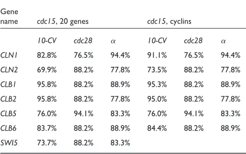
Examples of highly accurate rules are those created for genes
CLB1and CLB2(Table 2). The accuracy of the CLB1 classi-fier for ‘simultaneous’ events (Table 3, 20 genes) is 95.8% by the 10-fold cross-validation test along with 88.2% and 88.9% for the estimations where cdc28 and alpha-factor were used as test sets. It means that not only does cross-vali-dation produce highly accurate estimates, but the informa-tion extracted for CLB1from the cdc15dataset is consistent with the information about this gene contained in the cdc28
and alpha-factor datasets.
We can compare our classification rules with the analysis of expression time series, performed by Spellman et al. The authors evaluated and ranked all genes by a specific score. The better the score the more likely the gene is to be periodi-cally regulated. By establishing a threshold for the score values the authors identified cell-cycle-regulated yeast genes. Among those genes selected for our experiments there are eight that have scores lower than threshold defined by Spellman et al. These are SKP1, MBP1, CDC34, CDC53,
SWI6, HCT1, CDC28 and MCM1. We obtained no accurate rules for these genes, except for the questionable ones for
SKP1, MBP1and CDC34. All these questionable rules have high 10-fold cross-validation accuracy on cdc15data and are inconsistent with cdc28 and alpha-factor datasets. The reason for this is clear: these genes have much stronger signals during the cdc15experiment than during the other two (signal peak to trough ratio for cdc15is two or even three times higher than for cdc28 and alpha-factor datasets). The Table 1
The list of genes considered
ORF Gene name Description YMR199W CLN1 Cyclin, G1/S-specific YPL256C CLN2 Cyclin, G1/S-specific YAL040C CLN3 Cyclin, G1/S-specific YGR108W CLB1 Cyclin, G2/M-specific YPR119W CLB2 Cyclin, G2/M-specific YLR210W CLB4 Cyclin, G2/M-specific YPR120C CLB5 Cyclin, B-type YGR109C CLB6 Cyclin, B-type
YMR043W MCM1 Transcription factor of the MADS box family YLR079W SIC1 Inhibitor of Cdc28p-Clb protein kinase complex YLR182W SWI6 Transcription factor, subunit of SBF and MBF
factors
YBR160W CDC28 Cyclin-dependent protein kinase
YDL132W CDC53 Controls G1/S transition, component of SCF-ubiquitine ligase complexes
YDL056W MBP1 Transcription factor, subunit of the MBF factor YDR054C CDC34 E2 ubiquitin-conjugating enzyme
YDR146C SWI5 Transcription factor
YDR328C SKP1 Core component of SCF-ubiquitin ligase complexes
YER111C SWI4 Transcription factor, subunit of SBF factor YGL116W CDC20 Cell division control protein
situation is rather different for CDC53, SWI6, HCT1, CDC28
and MCM1: their expression levels are not significantly dif-ferent across all three experiments. Their scores indicate that they can serve as negative controls and, indeed, no accu-rate rules were obtained for these genes. This fact reflects that our rule-extraction procedure performed well and that we did not extract rules randomly.
It should be noted that the size of the used training sets is relatively small for a machine-learning approach. Classifica-tion is an individual problem in the case of each gene, and the size of the training set sufficient to achieve good accuracy can vary from gene to gene. The advantage of our approach is that to make classification more precise one can just add new experimental data (expression profiles) to the dataset. We also plan to biuld an expert system for gene network reconstruction, based on the method presented here.
Discussion
To verify the biological relevance of our results we consider the expression of the genes in association with the consecu-tive phases of the cell cycle, G1, S, G2, M, M/G1, which are usually used in the literature. The highest-accuracy classi-fiers were obtained for the group of cyclins for which almost all possible known relations were reconstructed: +CLB5<==>+CLB6; +CLB6<==>+CLB5; ±CLB2<==>±CLB1; -CLB1<==>-CLB2; -CLB2<==>+CLN2; +CLN2<==>+CLN1 and +CLB6==>-CLB1; +CLB6==>-CLB2; ±CLB1==>⫿CLN2. Our rules are consistent with the knowledge that the maximum of CLB2 transcription is in G2 phase, whereas CLN1, CLN2,
CLB5and CLB6, whose expression patterns are very similar, all have their expression maximum in G1 [15,18]. The rules obtained are in agreement with CLB2 and CLB1 being expressed simultaneously in G2 [19]. Questionable rules, 앖앗CLN2<==>앖앗CLB5and -CLB2==>+CLN1, from the lower
comment
reviews
reports
deposited research
interactions
information
[image:5.609.58.552.109.485.2]refereed research
Table 2
Classification rules
Gene name ‘Simultaneous’ rules Supporting information ‘Time delay’ and ‘changes’ rules Supporting information
SWI5 -CLB1<==>-SWI5 [19] -
--CLB2<==>-SWI5 [33]
CLN1 +CLN2<==>+CLN1 [22] -
--CDC20<==>+CLN1
CLN2 -CLB2<==>+CLN2 [20] ±CLB1==>⫿CLN2 [20]
+SWI5<==>-CLN2 [18] [18]
CLB1 ±CLB2<==>±CLB1 [19] +CLB6==>-CLB1 [19]
앖앗CLB2<==>앖앗CLB1 [21]
CLB2 -CLB1<==>-CLB2 [19] +CLB6==>-CLB2 [19]
앖앗CLB1<==>앖앗CLB2 [21]
CLB5 +CLB6<==>+CLB5 [15] -
-CLB6 +CLB5<==>+CLB6 [15] -
-MBP1 ⫿CDC34<==>±MBP1 [34] 앖앗CDC34<==>앗앖MBP1 [34]
CDC34 +MBP1<==>-CDC34 [34] -
-SKP1 +MBP1<==>-SKP1 [15] 앖앗CDC34<==>앖앗SKP1 [35]
SWI5 - - 앖CLN2<==>앗SWI5 [18]
±CLB1==>±SWI5 [20]
-CLB1-CLN3==>+SWI5
CLN1 - - +SWI5==>-CLN1 [20]
-CLB2==>+CLN1
CLB5 - - 앖앗CLN2<==>앖앗CLB5 [18]
part of Table 2 have the same explanations (see Classifica-tion rules for explanaClassifica-tion of quesClassifica-tionable rules).
Rules that we obtained for the expanded set of genes do not conflict with the ones for cyclins. They confirm several addi-tional details about coordination of cyclin transcription with expression of genes involved in cell-cycle regulation. For example, transcription of SWI5 and CLB1 is G2/M specific and activated in late S phase; the expression pattern of SWI5
is similar to that of CLB1and CLB2and the peak of mRNA concentration of SWI5 is in G2 [20,21]. The following classification rules for CLN1, CLN2and SWI5are in agree-ment with these data: +SWI5<==>-CLN2, -CLB1<==>-SWI5, -CLB2<==>-SWI5 and questionable rules 앖CLN2==>앗SWI5, +SWI5==>-CLN1.
Clearly, ‘simultaneous’ as well as ‘changes’ rules for MBP1
and CDC34, SKP1 (Table 2, lower part) can be explained by the fact that their activities as parts of the MBF and SCF complexes are completely separated in time.
The classification rules for CLN1 are: +CLN2<==>+CLN1, -CDC20<==>+CLN1. CDC20is transcribed in late S/G2 phase and its product is required for metaphase-to-anaphase tran-sition [20,22], whereas CLN2 and CLN1 have their tran-scription maximum in G1.
At the same time, there is a group of eight genes for which no accurate classifiers were obtained. There are several possible reasons for this and we discussed some in Classification rules. One obvious restriction of the microarray methodol-ogy is that it gives us information about gene regulation only at the level of transcription. Furthermore, mRNA extractions in the cdc15experiment were made every 10 minutes during
three cell cycles, which may not be frequent enough to observe all events. The sensitivity of microarray experiments is insufficient to see minor fluctuations of expression. For example, some of the selected genes are expressed at a low and nearly constant level, making the detection of slight changes in mRNA concentrations difficult. CDC28 is assumed to be expressed constitutively, as it is involved in all cell-cycle phases. It is required for initiation of mitosis, DNA replication, polarization of the actin cytoskeleton, spindle-pole-body duplication and bud emergence [23-26]. Further-more, most of the regulatory interactions of CDC28 are at the protein level, which cannot be straightforwardly detected by the microarray experiments considered. The data-quality issues in the context of gene-network reconstruction are dis-cussed in [2].
There are a few rules among those extracted that reflect symmetric relations between genes, and which, therefore, can be potentially obtained by clustering. For instance,
CLB1 and CLB2 rules are symmetric reflections of each other. However, the majority of extracted rules have a structure that is sufficiently different from the clustering-like one. Dependencies between explaining and predicted genes of the decision trees, from which the rules were con-structed, are even more complex and hardly can be retrieved by clustering algorithms (for decision trees see Additional data files).
The relationships between genes discussed here have simple biological meaning. These relationships may not be the optimal for constructing the full network of gene interac-tions; nevertheless, they exist in the data and may be clearly explained with the help of existing knowledge. Using the obtained results we can construct networks of gene inter-relationships by connecting genes by directed edges accord-ing to classifiers. Classifiers in such a network are considered to be the control functions, which map the expression levels of other genes into the state of a corre-sponding gene.
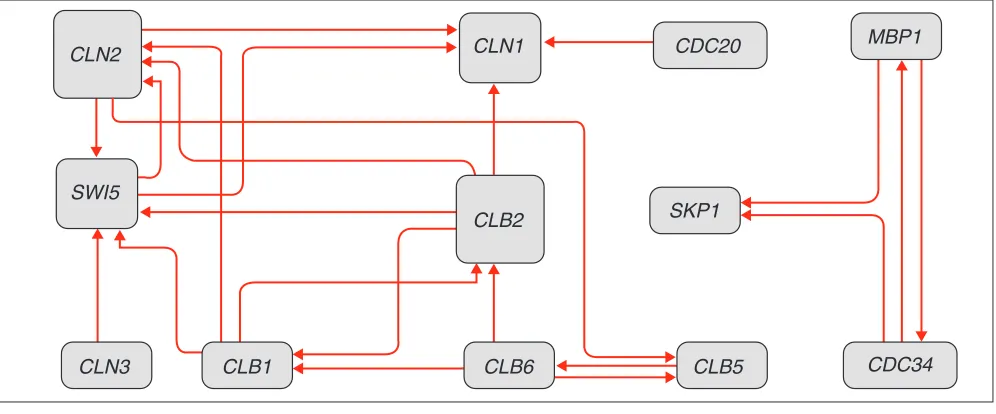
Connecting genes from Table 2 gives us the network pre-sented in Figure 2, which is simply a graphical representa-tion of the dependencies between gene-expression levels contained in the extracted decision rules. Every node in this graph represents a gene, and every arc indicates the relation between genes defined by the corresponding decision rule.
[image:6.609.55.296.127.278.2]An advantage of network reconstruction using our approach is that, given accurate classifiers, one is able to construct a network correctly, reproducing the architecture and the logic of a network consistent with the data. Moreover, one can easily improve classifiers by adding new expression profiles to the dataset. It is important that such iterative improve-ments can be part of an interactive process, when the researcher decides when to stop adding new data and what biological meaning is comprised in the network. Thus, our Table 3
Accuracy of final classifiers for ‘simultaneous’ events in the cdc15dataset
Gene
name cdc15, 20 genes cdc15, cyclins
10-CV cdc28 ␣ 10-CV cdc28 ␣
CLN1 82.8% 76.5% 94.4% 91.1% 76.5% 94.4% CLN2 69.9% 88.2% 77.8% 73.5% 88.2% 77.8% CLB1 95.8% 88.2% 88.9% 95.3% 88.2% 88.9% CLB2 95.8% 88.2% 77.8% 95.0% 88.2% 77.8% CLB5 76.0% 94.1% 83.3% 76.0% 94.1% 83.3% CLB6 83.7% 88.2% 88.9% 84.4% 88.2% 88.9% SWI5 73.7% 88.2% 83.3%
methodology can be considered as a basis for an interactive expert system for gene-interaction network reconstruction.
Conclusions
All the extracted classification rules are consistent with the data reported in the literature and even though the selected microarray experiments were not designed specifically for gene-network reconstruction, we were still able to find several features of gene transcriptional activities.
Although here we apply our approach to a relatively small subset of genes, it seems likely that it can be applied to larger gene sets. Time-course data are not the only type of data to which our approach is applicable. It is possible to explore various cases where potential dependencies between dif-ferent experimental samples might occur. A future goal is to use the method described to deduce larger gene-interac-tion networks and to investigate groups of genes with unknown interactions. We also plan to build an expert system for gene-network reconstruction, based on the method presented here.
Materials and methods
First, we give more formal definitions and formulations of the problems informally introduced in Definitions. The columns yj = (x1j,…,xkj) of the gene-expression matrix X
are called sample expression profiles. We also define a partial expression profile yj/i, where the expression value of gene iis missing. As already discussed, we assume that the transcription machinery of gene i can be in a finite
number of different states sijfor sample j. More precisely, we define the state function ifor an arbitrary given gene I
as a function such that given a real value x it returns a value from a discrete domain. Let us assume here that iis a function, which returns ‘+1’ if gene iis ‘upregulated’ (xij >—xi) and ‘-1’ if it is ‘downregulated’ (xij <—xi), where —xi is the average expression value of gene i. Thus, in this particular case i(x) 僆{-1,+1}. Given the expression value xijof gene
i, and the function i, we can define the state of the gene as sij = i(xij).
Our goal is, given a gene-expression matrix Xand a gene i, to predict: one, the state of the gene iunder condition jfrom the expression values of other genes in the same sample (that is, from the partial expression profile yj/i); two, the state of the gene iunder condition jfrom the expression values of genes from the previous sample/samples (that is, from the partial expression profile yj-1/i); three, the change in the state of the gene from the changes in states of other genes.
These three problems can be considered as standard classifi-cation problems in the following way. Let Y = {y1,…,yn} be the set of all sample expression profiles and Y/i={y1/i,…,yn/i} be the set of partial sample expression profiles for the given gene ifrom matrix X. Let us define a classifier, C, as a func-tion that maps a vector yto a discrete value s. Sometimes, in the context of classification, vector y is called a feature vector, while sis a label. The subset of y vectors with correct labels assigned to them is called a dataset, D, for a particular classification problem. An induction algorithm I maps a dataset D into a classifier C. Thus, to solve the problems above we need to define datasets and then choose appropriate
comment
reviews
reports
deposited research
interactions
information
[image:7.609.58.556.88.295.2]refereed research
Figure 2
The network of gene interactions constructed using the decision rules for the cdc15dataset (see Table 2). The network is a graphical representation of the information comprised in the extracted decision rules. Every node in this graph represents a gene and every arc indicates the relation between the genes defined by the corresponding decision rule. Note the existence of two separate modules in the constructed network.
CLN2
SWI5
CLN3
CLB1
CLB6
CLB5
SKP1
CLB2
CLN1
CDC20
MBP1
induction algorithms. Now we can formulate the three prob-lems more precisely.
We want to predict the state of gene lfrom matrix X. Induction algorithm Imaps the dataset Dl = (Y
/l,sl), into the classifierCl.
(We use index lfor Dland Clin order to emphasize that they
correspond to the lth gene.) For the given dataset Dl, we
want to create a classifier that predicts the state of gene l cor-rectly, that is, I(Dl,y
j/l)= Cl(yj/l)= slj. For the first problem,
the predicted gene land the explaining genes belong to the same sample j.
Formulation of the second problem is the same, except that the dataset now is Dl= (Yⴕ/l, sⴕl), where Yⴕ/l = {y
1/l,…,yn-1/l}
and sⴕl = (sl2, …, sln). The classifier Clis said to classify gene l
for sample j correctly, if Cl(y
j/l) = slj+1. Note that for this
problem the explaining genes belong to the sample preced-ing the sample of the predicted gene g.
To define the third problem we construct a matrix D consist-ing of elements dij = sij+1-sij, where sij = i(xij). The formula-tion of the third problem is equivalent to that of the first if we use dijinstead of xijand consider the pair (Y/l, dl) as the dataset for the third problem. Note that now yj/l = (d1j,…,dl-1 j,
dl+1 j, …, dkj) and dlis the row from the new matrix of dij
values associated with the predicted geneg. As a result, fea-tures and labels in this particular case belong to the same domain {-1,0,+1}, where ‘+1’ means that gene changed its state from ‘downregulated’ to ‘upregulated’, ‘-1’ means the opposite change and ‘0’ is used for the situation when the gene’s state remained unchanged in the transition from one sample (experimental condition) to another.
To solve the first two problems defined above, we have to use classifiers for continuous data, that is, any discretization should be a part of the classification algorithm. This enables us to find abundance thresholds of explaining genes, which are specific for different gene interactions in the network and sufficient for the switching of the predicting gene from one state to the other. This way every gene has its own unique discretization thresholds for input signals.
As a part of the classification problem it is necessary to find which genes are relevant to the prediction of a particular gene. This is known as the feature subset selection problem. Two kinds of methods for feature subset selection have been generally presented in the literature - filter and wrapper methods [16,17]. In the filter approach, the feature set is fil-tered to find the ‘most promising’ subset by evaluating some objective function before running the induction algorithm. The weak point of this approach is that the properties of a particular induction algorithm are ignored. In the wrapper approach, the selection algorithm uses the induction algo-rithm itself to evaluate the objective function. The wrapper approach of Kohavi was reported as performing better than the filter approach for many real and artificial datasets [17].
The idea of the wrapper algorithm is to tune parameters of an induction algorithm assuming it to be a black box in order to optimize some objective function (for example, the accuracy of a classifier). The set of attributes relevant to classification may be considered as parameters of an induction algorithm. Selecting the parameters that maximize the objective func-tion gives us a list of ‘good’ features. For the details of the selection algorithm see Kohavi [17]. The classification rules that we obtain support the validity of the assumption that only a limited number of explaining genes are sufficient for accurate predictions.
In this paper we use two types of induction algorithms. The first exploits the wrapper approach for feature subset selec-tion [17]. This one is C4.5 by Quinlan [27], with wrappers by Kohavi [17]. The second is C4.5 itself. C4.5 is an algorithm that constructs the classification model inductively, general-izing information from given examples of correct classifica-tion, and was selected as an algorithm of proven performance for a large variety of datasets.
We compared two different strategies for discretization. In the first, the data prediscretized by an entropy-based scheme with Fayyad and Irani stopping criteria [28] were used in the inducer with wrappers. This supervised discretization tech-nique uses the information entropy of the partitions induced by different thresholds to find the appropriate discretization boundaries, and it stops the search following the stopping criterion based on the so-called minimum description length principle (MDL) [16]. Thus the information entropy is used as the objective function in the search for the best splitting boundaries and, as the inductive splitting procedure requires some termination conditions, MDL is used as a criterion for termination. Because C4.5 was constructed as an algorithm that can be applied to continuous data [27], in the second approach we used C4.5 without additional discretization techniques. In addition, as used by Kohavi and Sahami [29], C4.5 can be used as an alternative to the Fayyad and Irani method for data discretization. All the classifiers were con-structed with the help of the WEKA package of machine-learning tools [30].
The main reasons for selecting the classification techniques described above are that their results (in the form of decision trees) are easy to interpret, they are algorithmically simple and there exist numerous comparisons of their performance in the literature. Moreover, these techniques have become benchmark algorithms for different machine-learning studies. Although each classification problem requires several classification techniques to be compared, and it is possible that more sophisticated and efficient induction algorithms exist for the datasets we used (although this is not proven), comparative analysis of induction algorithms and their development are not the topics of this study. The reader may consult the excellent studies of Kohavi [17] and Lim et al.
All the algorithms were run with default settings in order to use the results of comparisons of induction algorithms already reported in the literature and to avoid the additional bias associated with the tuning of parameters.
The accuracy estimates shown in Table 3 are for those ‘simultaneous’ events classifiers for which the performance of classifiers on the test sets is high. The table presents estimates for C4.5 with wrappers on the data predis-cretized by the Fayyad and Irani method. The accuracy of all extracted classifiers is presented in the additional data files. Because of the high variability of the estimates for cross-validation, it was repeated 30 times for different random partitions of the training sets for each selected classifier and the average values are shown. As two inde-pendent test sets were used, the cross-validation accuracy estimates serve only as an additional indicator of the per-formance of the created classifiers.
As the number of training instances is small, estimating the confidence limits for the accuracy mean is not straight-forward. Moreover, as has been pointed out by many researchers [17,32], the common assumptions concerning independence of different estimates are violated when cross-validation is used. In the presence of two indepen-dent test sets we did not do a rigorous analysis of stability of the classifiers, but, nevertheless, we observed that most of the final classifiers (not the questionable ones) were stable under different 10-fold splits. As is common prac-tice, cross-validation estimates are given along with stan-dard deviations. At the same time, 95% confidence intervals are shown for the accuracy estimates when the test sets were used. As the number of instances is small in both cdc28 and alpha-factor test sets, standard methodol-ogy based on the normal approximation of the binomial distribution is not applicable here. Instead, we estimated confidence intervals with the help of the Beta probability distribution using the methodology proposed in [32].
Additional data files
The following additional data files are available with the online version of this paper.
Additional data file 1 is a list of the classifiers for C4.5 by Quinlan with ‘wrappers’ by Kohavi on the cdc15dataset with continuous features discretized by the Fayyad and Irani method.
The first three tables in additional data file 1 present the classi-fiers for the set of 20 genes and the last three for the set of cyclins. The notation ‘simultaneous’ is used for the classifiers corre-sponding to the first problem, ‘time delay’ to the second problem, ‘changes’ to the third problem (see Definitions above). Addi-tional data file 2 is a list of the classifiers for C4.5 by Quinlan on the cdc15dataset with continuous features discretized by C4.5 itself. The content is organized as in additional data file 1.
Additional data file 3 contains accuracy estimates for the classifiers provided in additional data file 1.
Abbreviations: 10-CV, 10-fold cross-validation; cdc28 and ␣, accuracy estimates where cdc28 and alpha-factor datasets were used as test sets; Overall, test accuracy that was esti-mated by forming the unified cdc28-alpha-factor test set and testing the classifiers on it.
Cross-validation estimates are presented only for the classi-fiers from Table 2 to discriminate them from the others. Bold font is used for the final rules, excluding the question-able ones, and normal is used for the questionquestion-able rules. Cross-validation estimates are shown along with the stan-dard deviations, while 95% confidence intervals are pre-sented for those estimates where the test sets were used. Test accuracy was estimated under the assumption that the measurements of the cdc28 and alpha-factor test sets are independent. Additional data file 4 contains accuracy esti-mates for the classifiers provided in additional data file 2. The content is organized as in additional data file 3.
Acknowledgements
L.A.S. is supported by a grant from AstraZeneca. The WEKA package dis-tributed under the GNU General Public License was used for classifier creation and accuracy estimation. We thank Helen Parkinson, Johan Rung and Misha Kapushesky for useful discussions and the anonymous referees for their valuable comments.
References
1. van Berkum NL, Holstege FC: DNA microarrays: raising the profile.Curr Opin Biotechnol2001, 12:48-52.
2. D’haeseleer P, Liang S, Somogyi R: Genetic network inference: from co-expression clustering to reverse engineering. Bioin-formatics2000, 16:707-726.
3. Pe’er D, Regev A, Elidan G, Friedman N: Inferring subnetworks from perturbed expression profiles. Bioinformatics 2001, 17 (Suppl 1):S215-S224.
4. Akutsu T, Miyano S, Kuhara S: Algorithms for inferring qualita-tive models of biological networks.Pac Symp Biocomput 2000, 293-304.
5. Friedman N, Linial M, Nachman I, Pe’er D:Using Bayesian net-works to analyze expression data.J Comput Biol2000, 7:601-620 6. Kauffman SA: Metabolic stability and epigenesis in randomly
connected nets.J Theor Biol 1969, 22:437-467.
7. Chen T, He HL, Church GM: Modeling gene expression with differential equations. Pac Symp Biocomput 1999, 29-40. [http://www.smi.stanford.edu/projects/helix/psb99/Chen.pdf] 8. D’haeseleer P, Liang S and Somogyi R: Tutorial on gene
expres-sion data analysis and modeling. Pac Symp Biocomput 1999. [http://psb.stanford.edu/psb99/genetutorial.pdf]
9. Spellman PT, Sherlock G, Zhang MQ, Iyer VR, Anders K, Eisen MB, Brown PO, Botstein D, Futcher B: Comprehensive identification of cell cycle-regulated genes of the yeast Saccharomyces cerevisiae by microarray hybridization. Mol Biol Cell 1998, 9: 3273-3297.
10. Cho RJ, Campbell MJ, Winzeler EA, Steinmetz L, Conway A, Wodicka L, Wolfsberg TG, Gabrielian AE, Landsman D, Lockhart DJ, Davis RW: A genome-wide transcriptional analysis of the mitotic cell cycle. Mol Cell1998, 2:65-73.
11. Brazma A, Hingamp P, Quackenbush J, Sherlock G, Spellman P, Stoeckert C, Aach J, Ansorge W, Ball CA, Causton HC, et al.: Minimum information about a microarray experiment (MIAME) - toward standards for microarray data.Nat Genet 2001, 29:365-371.
comment
reviews
reports
deposited research
interactions
information
12. Quackenbush J: Computational genetics: computational analysis of microarray data.Nat Rev Genet 2001, 2:418-427. 13. PubMed [http://www.ncbi.nlm.nih.gov/entrez/query.fcgi] 14. YPD
[http://www.proteome.com/databases/YPD/YPDsearch-quick.html] 15. Chen KC, Csikasz-Nagy A, Gyorffy B, Val J, Novak B, Tyson JJ:
Kinetic analysis of a molecular model of the budding yeast cell cycle.Mol Biol Cell2000, 11:369-391 .
16. Witten I, Frank E: Data Mining - Practical Machine Learning Tools and Techniques with JAVA Implementations. San Francisco, CA: Morgan Kaufmann; 1999.
17. Kohavi R: Wrappers for performance enhancement and oblivious decision graphs. PhD thesis, Stanford University, Computer Science Department, 1995.
[http://robotics.stanford.edu/~ronnyk/ronnyk-bib.html]
18. Schneider BL, Patton EE, Lanker S, Mendenhall MD, Wittenberg C, Futcher B, Tyers M: Yeast G1 cyclins are unstable in G1 phase. Nature1998, 395:86-89.
19. Althoefer H, Schleiffer A, Wassmann K, Nordheim A, Ammerer G: Mcm1 is required to coordinate G2-specific transcription in Saccharomyces cerevisiae.Mol Cell Biol1995, 15:5917-5928. 20. Loy CJ, Lydall D, Surana U: NDD1, a high-dosage suppressor of
cdc28-1N, is essential for expression of a subset of late-S-phase-specific genes in S. cerevisiae.Mol Cell Biol1999, 19:3312-3327.
21. Toyn JH, Johnson AL, Donovan JD, Toone WM, Johnston LH: The Swi5 transcription factor of Saccharomyces cerevisiaehas a role in exit from mitosis through induction of the Cdk-inhibitor Sic1 in telophase.Genetics1997, 145:85-96.
22. Hwang LH, Lau LF, Smith DL, Mistrot CA, Hardwick KG, Hwang ES, Amon A, Murray AW: Budding yeast CDC20: a target of the spindle checkpoint.Science 1998, 279:1041-1044.
23. Reed SI, Wittenberg C: Mitotic role for the CDC28 protein kinase of Saccharomyces cerevisiae. Proc Natl Acad Sci USA 1990, 87:5697-5701.
24. Cvrckova F, Nasmyth K: Yeast G1 cyclins CLN1 and CLN2and a GAP-like protein have a role in bud formation. EMBO J 1993, 12:5277-5286.
25. Benton BK, Tinkelenberg AH, Jean D, Plump SD, Cross FR: Genetic analysis of Cln/CDC28 regulation of cell morphogenesis in budding yeast.EMBO J1993, 12:5267-5275.
26. Jaspersen SL, Charles JF, Morgan DO: Inhibitory phosphorylation of the APC regulator Hct1 is controlled by the kinase CDC28 and the phosphatase Cdc14.Curr Biol1999, 9:227-236. 27. Quinlan JR: C4.5: Programs for Machine Learning. San Francisco, CA:
Morgan Kaufmann; 1992.
28. Fayyad U, Irani K: Multi-interval discretization of continuous-valued attributes for classification learning. In Proceedings of the Thirteenth International Joint Conference on Artificial Intelligence. San Mateo, CA: Morgan Kaufmann; 1993: 1022-1029.
29. Kohavi R, Sahami M: Error-based and entropy-based dis-cretization of continuous features. In Proceedings of the Second International Conference on Knowledge Discovery and Data Mining. Edited by Simoudis E, Han J, Fayyad U. Menlo Park, CA: The AAAI Press; 1996: 114-119.
[http://www.aaai.org/Press/Proceedings/KDD/1996/kdd96.html] 30. WEKA [http://www.cs.waikato.ac.nz/~ml/weka]
31. Lim T-S, Loh W-Y, Shih Y-S: A comparison of prediction accu-racy, complexity, and training time of thirty-three old and new classification algorithms. Machine Learning, 2000, 40:203-228.
32. Martin JK, Hirschberg DS: Small sample statistics for classifica-tion error rates ii: confidence intervals and significance tests.Technical Report No. 96-22. Irvine, CA: University of Califor-nia, Irvine; 1996. [http://www.ics.uci.edu/~dan/pub.html]
33. Koranda M, Schleiffer A, Endler L, Ammerer G: Forkhead-like transcription factors recruit Ndd1 to the chromatin of G2/M-specific promoters.Nature 2000, 406:94-98.
34. Goebl MG, Goetsch L, Byers B: The Ubc3 (Cdc34) ubiquitin-conjugating enzyme is ubiquitinated and phosphorylated in vivo. Mol Cell Biol1994, 14:3022-3029.