Decision making Method for an Ordered Information System Based on Multi granulation Rough Sets

2018 International Conference on Computer Science and Software Engineering (CSSE 2018) ISBN: 978-1-60595-555-1

Decision-making Method for an Ordered

Information System Based on

Multi-granulation Rough Sets

Jiajia Zhang, Zhengkui Lin, Xuesheng Liu and Qing Dai

1

ABSTRACT

In this paper, we study an ordered problem of objects with multi-attributes based on granulation computing (GrC) for an ordered information system (OIS) and develops a novel multi-granulation rough set (MGRS) named the compromise multi-granulation rough set (CMGRS). The CMGRS is a generalized model of the classical MGRS. This new tool has a good weak transitivity and can be used to address ordered problems of objects in an OIS. Based on this novel MGRS, we construct a new approach for the ordered problem of objects for an OIS. This research introduces a method and discusses its characteristics. The results from an example investment project and the 2007 sustainability report indicate that our new approach is significant and efficient and achieves optimal results.

INTRODUCTION

In general, an information system (IS) with multi-attribute decision objects and a partial ordering of the attribute domain is called an ordered information system (OIS). Many decision problems represent ranking problems for an OIS. The ranking problem is an important branch of the decision problem. The OIS is not a serially ordered set; thus, many ranking methods are proposed [1].

Jiajia Zhang1, Zhengkui Lin1, Xuesheng Liu 2 and Qing Dai1,

1

Shipping Economy and Management College, Dalian Maritime University, Dalian, China, 116026

2

In practical problems, data may have preference information as well as inaccurate and ambiguous information. In such a scenario, the classic rough set method is not adequate. To handle information systems with partial ordering relationships, Greco [2] proposed a rough set model based on dominant relationships instead of equivalent relationships. In recent years, because of the rough set model’s many advantages, it has been widely used for the sequencing problem of the OIS. Many scholars have conducted a series of studies on ranking methods based on dominant relationships. Li et al. [3] presented a possibility ranking method with a superior degree matrix. According to the research of the ranking methods in an incomplete interval valued IS, Zhang et al. [4] proposed a ranking method with an improved possibility degree dominant relationship to solve the problem in which too many attributes may result in the ranking’s failure. This ranking method combined the interval-valued dominant relationship with the possibility degree, improved the weakness of the definition of the classic dominant relationship and defined the average comprehensive dominance degree. Moreover, the structure of the advantage matrix satisfies the complementary symmetry. Additionally, a method that accounts for the relative dominance degree was proposed by Duan et al. [5] for the multi-granularity rough set based on a dominant relationship. As IS research deepens, scholars have begun to focus on the attribute value of the object, which is fuzzy. To conduct decision analyses in a fuzzy situation, many scholars have begun to research ranking methods based on fuzzy sets. Wang et al. [6] proposed a multi-attribute decision-ranking method under the intuitionistic fuzzy environment combined with the intuitionistic fuzzy weighted average operator. The calculation formulas of the centroid positioning of the polygonal fuzzy number and the criterion of the index ranking were proposed by Wang et al. [7]. Then, according to the centre-weighted average rule and the horizontal and vertical centre formula of a trapezoidal fuzzy number, these authors [8] proposed an index ranking method.

MULTI-GRANULATION ROUGH SET OF A CLASSICAL ORDERED INFORMATION SYSTEM [10].

The optimistic and pessimistic MGRSs are defined by multiple dominant relationships in the OIS.

Definition 2.1. A ternary is an OIS in which is a non-empty

finite set of objects called the universe; is a non-empty finite set of attributes, and a dominant relationship is induced by a partial ordering that exists in the domain of each attribute; and is a mapping from to , and , where

is the finite domain of attribute .

Definition 2.2. Let be an OIS, , and be an

attribute set. are the dominant relationships, and . The

multi-granulation lower and upper approximation operators of of the OIS are defined by

(1)

₍₂₎

where , is a power set of , and is called the dominating class of

the dominant relationship in each of .

Similarly, the pessimistic multi-granulation lower and upper approximation operators of _{of the OIS are defined as follows:}

(3)

₍₄₎

Based on the above descriptions, a target concept can be approximated by using two different approximating strategies: seeking the common reserving difference and seeking the common rejection difference in the optimistic and pessimistic MGRSs of the classical OIS. We also construct the structure of the granular space of the target concept [11].

In many practical problems, decision makers must take advantage of available decision information with many complex decision environments. Therefore, the classical MGRS must be extended. In the following, we will extend the classical MGRS to compose the CMGRS of the OIS.

(U,AT,F)

I≥= _U

AT

F U Va F={fU→Va,a∈AT}

a

V a

(U,AT,F)

I≥=

AT A A

A1, 2,, s⊆ AT

≥ ≥ ≥

s

A A

A R R

R₁, ₂,, X∈P(U)

X

( )

(

[ ]

)

   

 

⊆ =

∑

≥

= ≥

∨

=

X x x X

OM s _i

i i

A s

i A

1 1

( )

(

[ ]

)

   

 

≠ =

∑

≥

= ≥

∧

=

φ

X x x X OM

i s

i i

A s

i

A ∩

1 1

AT

S≤2 P(U) U [ ]≥

i

A

x Ai

-≥

i

A

R Ai AT

X

( )

(

[ ]

)

   

 

⊆ =

∑

≥

= ≥

∧

=

X x x X PM

i s

i i A

s

i A

1 1

( )

(

[ ]

)

   

 

≠ =

∑

≥

= ≥

∨

=

φ

X x x X PM

i s

i i

A s

i

A ∩

COMPROMISE MULTI-GRANULATION ROUGH SET OF OIS

Definition 3.1. Let be an OIS, , and be an attribute set.

represents attributes of _{, where} . For an arbitrary

group of attributes that can be written as , are the

dominant relationships. Moreover, for , the CMGRS of the lower approximation and upper approximation of with respect to is denoted by

and , respectively, where

(5) (6)

and where .

Theorem 3.1.

If , then , .

If , then , .

Proof: Let . From Definition 3.1, the following is easily derived:

and .

Let . To prove , we need to prove and

.

Now, we prove that .

, i.e., ; therefore, is not included in and

can be obtained. Thus, , or . Hence,

. Then, we prove that . If (i.e.,

) and , then is not observed in which .

Moreover, can be obtained. Thus, , such that

.

In summary, can be obtained, which is similar to the proof of

. This completes the proof. (U,AT,F)

I≥= A₁,A₂,,A_s⊆AT AT

(AT)

Pr r Ai1,Ai2,Air AT ( )

r AT

r AT C

P =

r

i i

i A A

A, ,

2

1 ATr⊆AT

≥ ≥ ≥ r i i

i A A

A R R

R , , ,

2 1

( )U P

X∈

X P( )U

( )X CMAT_r

≥ _{CM ( )X}

r AT ≥ ( )

(

[ ]

)

      ⊆ = _∧ =

≥ _{X x x X}

CM k i r A r k AT 1 ( )

(

[ ]

)

      ≠ = _∨ =

≥ _{X x x X φ}

CM k i r A r k AT ∩ 1 ( )

{ P AT }

i∈1,2,, r

AT

r= _{CM ( )X PM ( )X}

s i i r A AT ≥ ≥ ∑ = =1

( )X PM ( )X

CM s i i r A AT ≥ ≥ ∑ = =1 1 =

r _{CM ( )X OM ( )X}

s i i r A AT ≥ ≥ ∑ = =1

( )X OM ( )X

CM s i i r A AT ≥ ≥ ∑ = =1 AT r=

( )X PM ( )X

CM s i i r A AT ≥ ≥ ∑ = =1

( )X PM ( )X

CM s i i r A AT ≥ ≥ ∑ = =1 1 =

r _{CM ( )X OM ( )X}

s i i r A AT ≥ ≥ ∑ = = = 1 1

( )X OM ( )X

CM s i i r A AT ≥ ≥ ∑= = ⊆ 1 1

( )X OM ( )X

CM s i i r A AT ≥ ≥ ∑₌ = ⊇ 1 1

( )X OM ( )X

CM s i i r _A AT ≥ ≥ ∑ ⊆ = = 1 1

( )X OM

x s

i Ai

≥

∑

∈ ∀

=1

~ ∀Ai,i=1,2,,s [ ] ≥

i

A

x X [ ]x X

i

A⊄

≥

( )X CM x r AT ≥ = ∈ 1

~ _{OM ( )X CM ( )X}

r s

i Ai AT

≥ ≥ = = ⊆ ∑ 1 1 ~ ~

( )X OM ( )X

CM s i i r A AT ≥ ≥ ∑ ⊆ = = 1

1 CM ( )X OM s ( )X

i i r _A AT ≥ ≥ ∑ ⊇ = = 1 1

( )X CM x r AT ≥ = ∈

∀ ~ ₁

( )X CM

x∉ AT≥_r=1 ∀Ai,i=1,2,,s [ ]xAi⊆X

≥ _i=1,2,,s

( )X OM

x s

i Ai

≥

∑ ∈

=1

~ OM s ( )X CM r ( )X

i Ai AT

≥ ≥ = = ⊇ ∑ 1 1 ~ ~

( )X OM ( )X

CM s i i r A AT ≥ ≥ ∑ ⊇ = = 1 1

( )X OM ( )X

CM s i i r A AT ≥ ≥ ∑ = =1

( )X OM ( )X

Definition 3.2 Let be an OIS. Then, we can define a dominant class in which all objects are at least as good as the object with respect to the attributes in the universe. This class is written as , although it is occasionally written

as .

_{[ ] [ ]}

{

_{j A ( )i A}

_{( )}

_{j A ( )i A}

_{( )}

_j

}

C i AT

i x x f x f x f x f x

x

r i r

i i

i r

r = = ≤ ≤

≥ ≥

, ,

1 1

(7)

where is the arbitrary attributes of the attribute set, such that the

object is at least as good as the object with respect to the attributes .

Theorem 3.2.

satisfies the following properties:

1) If for all attributes in , then is at least as good as , and then

.

2) If , then .

3) is a coverage of .

Proof: Items 1)-3) are easy to verify.

ORDERED METHOD OF CMGRS OF OIS

Based on the CMGRS, the OIS is converted to the model of the dominant relationship. The object results can be obtained by this model.

For the dominant classes and , we utilize the inclusion degree to

calculate a degree of superiority [12], where outranks with respect to the

attribute set .

( ) [ ] [ ]

U x x x x

R r r

r

AT j AT i j i AT

≥ ≥

=

∪ ~

, (8)

where represents the number of the elements of the set .

Theorem 4.1. satisfies the following properties:

1) ; 2) If , then ;

3) If , then ; 4) If , then .

Proof: 1) For , there are always . Thus, .

(U,AT,F) I≥=

i

x

r

AT [ ]≥

r

AT i

x

[ ]≥

r

C i

x

[ ]≥

r

AT i

x r

r

i i

i A A

A, , ,

2

1

j

x xi Ai1,Ai2,,Air

[ ]≥

r

AT i

x

[ ]iAT

j x

x ∈ AT xj xj

[ ]

≥ [ ]≥

⊆ i AT

AT

j x

x

ρ

<

r [ ]≥ [ ]≥ ⊇

ρ AT i AT

i x

x

r [ ]

{

x x U

}

J = i ATr i∈ ≥

≥ _U

[ ]≥

r

AT i

x

[ ]

≥

r

AT j

x

i

x x_j

r

AT

• xi,xj∈U

r

AT

R

( , ) 1

0≤RATr xi xj ≤ [ ]

≥ ∈ i _AT

j x

x RATr(xj,xi)=1 [ ]≥

∈ k _AT

j x

x RAT_r(xi,xj)≤RAT_r(xi,xk) [ ] ≥ ∈ k _AT

j x

x RAT_r(xj,xi)≥RAT_r(xk,xi)

j i,

∀

{

[ ]x

[ ]

x

}

U

r r j AT AT

i ⊆

⊆ ~ ≥ ∪ ≥

2) If , then . If such that

, then and . We can obtain

.

3) For , we can obtain from 2). By comparing

with , we obtain .

4) If , from the above proof, we have , and then .

By comparing with ,

can easily be obtained. This completes the proof.

By using the average number of each object, a synthetic degree of superiority is

calculated with respect to the attributes as follows: .

As the value of increases, object improves. We can rank all objects from big to small [13].

Theorem 4.2 Let be an OIS. Then, satisfies the following

properties: 1) ; 2) If , then .

Proof: 1) Obviously, 1) can be easily proved.

2) Now, we prove 2) by comparing with when . From 4) of

Theorem 4.1, we know that , . Moreover,

can be easily obtained such that . By comparing

with _{, we can obtain . The above information}

indicates that . This completes the proof.

From the above ranking approach, we obtain two points. One point is the pointed order, in which all attributes are better. The other point is that this approach utilizes third-party information to rank the objects for the dissatisfied pointed order. This approach ensures the principle of pointed order (i.e., that rationality is a main

principle and that whole attributes are better) and ranks the objects of the dissatisfied pointed order. This approach is effective. A ranking approach of the multi-attribute CMGRS of the OIS is verified by the following example.

Example 4.1. [12] Let represent an OIS of an investment

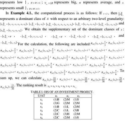
project as shown in table 1 of the supplementary material. is an attribute set, where , represents the location, represents the scale of investment, and represents the density of population. Figures in brackets represent the quantity change of the attribute value. represents good, represents average, and

[ ]≥ ∈ i _AT

j x

x fA₁( )xj ≥fA₁( )xi,,fA_s( )xj ≥fA_s( )xi

[ ]

≥ ∈ ∀

r

AT j

k x

x

( )k A( )j A( )i A( )k A ( )j A( )i

A x f x f x f x f x f x

f

r i r i r i i i

i1 ≥ 1 ≥ 1 , , ≥ ≥

[ ]≥ ∈

r

AT i

k x

x

[ ]

≥ ⊆[ ]≥

r r i AT

AT

j x

x

( j, i)=1

AT x x

R r

[ ]≥

∈ k AT

j x

x

[ ]

≥ ⊆[ ]≥

r r k AT

AT

j x

x

( ) [ ]≥ [ ]≥

=

r r r i j iAT jAT

AT x x

U x x

R , 1 ~ ∪ ( )= [ ]≥ [ ]≥

r r r i k iAT kAT

AT x x

U x x

R , 1 ~ ∪ RATr(xi,xj)≤RATr(xi,xk)

[ ]≥

∈ k AT

j x

x [ ]≥ [ ]≥

⊆

r r k AT

AT

j x

x [ ]≥ ⊇ [ ]≥

r r kAT

AT

j x

x ~

~

( j i)

AT x x

R

r , RATr(xk,xi) RATr(xj,xi)≥RATr(xk,xi)

r ( ) (i j)

j i

AT i

AT R x x

U x R

r

r ,

1

1 _∑

≠ − =

( )i

AT x

R

r xj

(U,AT,F) I≥=

( )i

AT x

R r ( ) 1

0≤RATr xi ≤ [ ]

≥ ∈

r

AT i

j x

x RATr( )xi ≤RATr( )xj

( )i

AT x

R

r RATr( )xj k≠i,k≠ j ( j i) AT( k i)

AT x x R x x

R

r

r , ≥ ,

[ ]

≥ ∈

r

AT j

j x

x

[ ]

≥ ⊆[ ]≥

r r i AT

AT

j x

x

[ ]

≥ [ ]≥ ⊇

r r i AT

AT

j x

x ~

~ _{( ) [ ]}≥ _{[ ]}≥

=

r r r i j iAT jAT

AT x x

U x x

R , 1 ~ ∪

( ) [ ]≥ [ ]≥

=

r r r j i jAT iAT

AT x x

U x x

R , 1 ~ ∪

(i j) AT( j i)

AT x x R x x

R

r

r , ≤ ,

( )i AT( )j

AT x R x

R _r ≤ _r

{x1,x2,x3,x4,x5,x6}

U=

AT

{a1,a2,a3}

AT= a1 a2

3

a

G Va1={

represents bad , ; represents high, represents average, and

represents low , ; represents big, represents average, and

represents small , .

In Example 4.1., the computational process is as follows: If , then

represents a dominant class of with respect to an arbitrary two-level granularity:

, , , , , and

. We obtain the supplementary set of the dominant classes of :

, , , , , and

.

For the calculation, the following are included: (₁, ₂) ₃1

2 x x =

R_AT , RAT2(x1,x3)=1

,

( )

3 2 , ₄

1

2 x x =

R_AT , ( )

2 1 , ₅

1

2 x x =

R_AT , ( )

3 2 , ₆

1

2 x x =

R_AT , RAT2(x2,x1)=1

, _{( , ) 1}

3 2 2x x =

RAT , RAT2(x2,x4)=1

, _{( , ) 1}

5 2 2x x =

RAT ,

(2, 6) 1

2 x x =

RAT , RAT2(x3,x1)=1

, _{( )}

3 1 , ₂

3

2 x x =

R_AT , ( )

3 2 , ₄

3

2 x x =

R_AT , ( )

2 1 , ₅

3

2 x x =

R_AT , ( )

3 2 , ₆

3

2 x x =

R_AT , RAT2(x4,x1)=1

,

( )

3 2 , ₂

4

2 x x =

R_AT , (₄, ₃) 1

2 x x =

R_AT , _{( )}

6 5 , ₅

4

2 x x =

R_AT , (₄, ₆) 1

2x x =

R_AT , (₅,₁) 1

2x x =

R_AT , _{( )}

6 5 , ₂

5

2 x x =

R_AT , ( ₅, ₃) 1

2x x =

R_AT ,

( ₅, ₄) 1

2x x =

R_AT , (₅, ₆) 1

2 x x =

R_AT , ( ₆, ₁) 1

2 x x =

R_AT , _{( )}

3 2 , ₂

6

2 x x =

R_AT , (₆, ₃) 1

2 x x =

R_AT , ( ₆, ₄) 1

2x x =

R_AT , _{( )}

6 5 , ₅

6

2 x x =

R_AT . To

sum up, we can calculate _{( )}

30 19

1

2 x =

R_AT , ( )₂ 1

2x =

R_AT , ( )

30 19

3

2 x =

R_AT , ( )

30 27

4

2 x =

R_AT , ( )

30 29

5

2 x =

R_AT ,

( )

30 27

6

2 x =

[image:7.612.99.498.105.507.2]

RAT . The ranking result is x2>x5>x4=x6>x1=x3.

TABLE I. OIS OF AN INVESTMENT PROJECT. U/AT a1 a2 a3

x1

x2

x3

x4

x5

x6

(1)B (2)M (1)S

(3)G (2)M (2)M

(1)B (1)L (2)M (2)C (1)L (3)B (2)C (3)H (2)M (2)C (2)M (1)S

EXAMPLE

Based on the data from the 2007 sustainability report (the data can obtain from zjj892177892@163.com), we conduct a ranking study of the capacity of regional sustainable development. The data are included in the supplement. From the index system, five indicators are used to determine the capacity of sustainable development. We assess the sustainability of 31 regions in our country. U={Beijing, Tianjin, Hebei, Shanxi, Neimenggu, Liaoning, Jilin, Heilongjiang, Shanghai, Jiangsu, Zhejiang, Anhui, Fujian, Jiangxi, Shandong, Henan, Hubei, Hunan, Guangdong, Guangxi, Hainan, Chongqing, Sichuan, Guizhou, Yunnan, Xizang, Shanxi, Gansu, Qinghai, Ningxia, and Xinjiang _{} { }}

31 2 1,x, ,x

x

= is an object set, and

} G≥C≥B Va2={H

M L

} H≥M≥L Va3={B M S

} B≥M≥S

2

=

r [ ]≥

2

C

x

x

[ ]x1C2={x1,x2,x3,x4,x5,x6}

≥ _{[ ] { }}

5 2 2 2 x,x

x ≥_C = _{[ ]}x3C2={x1,x2,x3,x4,x5,x6}

≥ _{[ ] { }}

6 5 4 2 4 2 x,x,x,x

x _C≥ = [ ]x5C2={x2,x4,x5}

≥

[ ]x6C2={x2,x4,x5,x6}

≥ _x

[ ]≥ =φ 2 1

~ x _C ~[ ]₂ {₁, ₃, ₄, ₆}

2 x x x x

x _C≥ = _{[ ]}≥ =φ

2 3

~ x _C ~[ ]x4C2={x1,x3}

≥

[ ]5 {1, 3, 6} ~

2 x x x x _C≥ =

[ ]6 {1, 3} ~

{

=

AT survival attribute index, developmental attribute index, environmental

attribute index, social support attribute index, and intelligence support system index } {= a1,a2,a3,a4,a5} is an attribute set. F is a mapping from U to Va_j. For each xi

and j

a

V , we have

j

j i a

a x V

F ( )= . Thus, a sustainable IS can be obtained. First, we

preprocess the data and use equal widths to discretize the data to facilitate data comparisons. Then, we use the method proposed in this paper for the calculations. We take r=3 _{in this example. MATLAB is used for the computations, and the}

following result is obtained:

.

29 24 26 30 28 4 25

5 12 31 20 23 22 27 14 16 17 7 18 3 21 6 13 15 10 8 19 11 2 9 1

x x x x x x x

x x x x x x x x x x x x x x x x x x x x x x x x

> > > > > > >

> > > = > > > > > > > > > > > > > > > > > > >

Using the average comprehensive dominance degree (ACDD) in [4], the result is as follows:

.

29 24 26 30 28 4

25 5 12 31 23 20 22 27 14 16 21 3 17 18 7 6 15 13 2 8 10 19 1 11 9

x x x x x x

x x x x x x x x x x x x x x x x x x x x x x x x x

> > > = > >

> > > = > > > > > > > > > > > > > > > > > > > >

A comparison with the ACDD method [4] shows that our method can better separate different target areas; thus, our method has a higher degree of differentiation. Our method is both effective and simple. The results show that Beijing has the strongest sustainable development and Shanghai presents the second strongest sustainable development, whereas Qinghai has the weakest sustainable development. Shanghai and Beijing are China's first-tier cities and represent economic centres; thus, these cities will have the strongest sustainable development, which is consistent with known data. However, in the ACDD, Shanghai has the strongest sustainable development and Zhejiang has the second strongest sustainable development. Thus, the sustainable development of Beijing is lower than that of Zhejiang, which is not consistent with known data. The weakest sustainable development is observed in the same city as that obtained using our method. Therefore, the experiment shows that our method is effective and practical.

CONCLUSIONS

ACKNOWLEDGEMENTS

This work is supported by the National Science Foundation of China (Nos. 61170255).

REFERENCES

1. Liu, Xuesheng, W. Wu, and J. Hu. 2008. "A method of fuzzy multiple attribute decision making

based on rough sets." J. International Journal of Innovative Computing Information & Control Ijicic, 4(8):2005-2010.

2. Greco, Salvatore, B. Matarazzo, and R. Slowinski. 2001. "Rough sets theory for multicriteria decision analysis." J. European Journal of Operational Research, 129(1):1-47.

3. Wei-Wei, L. I., Y. I. Ping-Tao, and Y. J. Guo. 2015. "New Reordering Method for

Comprehensive Evaluation and Solving Algorithm." J. Journal of Northeastern University,

36(4):606-608.

4. Zhang, Qi Wen, X. Q. Wang, and X. L. Zhuang. 2015. "Research of Ranking Method Based on

Improved Possible Degree Dominance Relation." J. Computer Science.

5. Duan, Yunyan, L. V. Yuejin, and F. Xie. 2017. "Ranking method of multi- granularity rough set

based on dominance relation and its application." J. Computer Engineering & Applications.

6. Wang, Zhong Xing, et al. 2013. "A New Scoring Function of Interval-valued Intuitionistic Fuzzy Number and Its Application in Multi-attribute Decision Making." J. Fuzzy Systems & Mathematics 27 (4):167-172.

7. Wang, Qin, et al. 2017. "Centroid positioning of the polygonal fuzzy number and its ordering method." J. Journal of Northeast Normal University.

8. Wang, Qin, et al. 2017. "Ordered Expression of Trapezoidal Fuzzy Number and the Center

Average Ranking Method." J. Operations Research & Management Science.

9. Intan, Rolly, and M. Mukaidono. 2003. "Multi-rough sets based on multi-contexts of attributes."

C. International Conference on Rough Sets, Fuzzy Sets, Data Mining, and Granular Computing Springer-Verlag, pp: 279-282.

10. Qian, Yuhua, et al. 2010. "MGRS: A multi-granulation rough set." J. Information Sciences,

180(6):949-970.

11. Xu, Weihua, et al. 2012. "Multiple granulation rough set approach to ordered information systems." J. International Journal of General Systems, 41(5):475-501.

12. W. Xu. 2013. "Ordered information system and rough set." Science Press.

13. Qiu, Guo Fang, et al. 2013. "A knowledge processing method for intelligent systems based on

inclusion degree." J. Expert Systems, 20(4):187-195.

14. Hu, Qinghua, Z. Xie, and D. Yu. 2007. "Hybrid attribute reduction based on a novel fuzzy-rough