Prediction Model for Road Traffic Accident Based on Support Vector

(1)

2018 3rd International Conference on Information Technology and Industrial Automation (ICITIA 2018) ISBN: 978-1-60595-607-7

Prediction Model for Road Traffic Accident

Based on Support Vector

Rong Cheng, Xiaoqiang Tian and Mengmeng Zhang

ABSTRACT

More than 1.3 million people worldwide die in road traffic accidents every year. With that in mind, traffic safety has become a top priority to the road traffic system development. Research in progress of road traffic accidents mainly from accidents numbers and the degree of accident damage. Firstly, this paper proposes a support vector prediction model for predicting the amount of road traffic accidents, which applied to the actual to verify the validity of the model by using the R software to solve it. Finally, it is found to the problem on a small scale has a better prediction effect which for the support vector model by comparing with the random forest model.1

KEYWORDS

Traffic Accident; Prediction Model; Support Vector

INTRODUCTION

Road traffic safety has become a global social problem. It is estimated that currently more than 3,000 people global, and nearly 1.30 million people each year died in road traffic accidents, and another 20 million to 50 million people were injured or disabled due to collisions caused by road traffic accidents. Traffic safety problems caused by traffic accidents have become a serious social problem, it is

(2)

measures to suppress the occurrence of accidents, which according to the impact of traffic the various factors of safety analyze the relevant data2.

SVRPREDICTION MODEL

It researched on the amount of the traffic accidents, which the traditional statistical models commonly included that linear regression models, Poisson regression models, negative binomial distribution models, zero-inflated model and Hurdle models. The following elaborated support vector expressions, features and in which using condition.

The basic idea of the Support Vector Regression Model (SVR) 3is to map the training set datafunctions Φ of the input space into the higher dimensional features space, then construct a separate hyperplane with the large margin principle for the feature space. Given training set data , 1, 2, , ,

n i

x R i l

and l represents magnitude which of the training and the data, yi  1 _,SVM ₄_making

 

0

f x   x  b

for positive examples ,and f x

 

 

 

x  b 0for negative examples, which making by the hyperplane direction  and the offse scalar b .Therefore, even though we didn’t find linear function in the input space to determine the type of the given data, but we can easily find an optimal hyperplane which clearly distinguishes the two data types.

Given the training data set





x y1, 1



, ,



x yl, l





_{,of which}

n i

x R

represents the input space of the sample for each i1, 2, ,l can find yi R_{.The idea of the}

regression problem which is to find a function that can determine a more accurate prediction of future values. SVR estimation function takes the following form generally:

 



 



f x   x b

 

1

Where Rn, bR , Φ represents a nonlinear transformation from a high-dimensional space. If we want find the values of and b that determine the value of x by minimizing the regression risk.

2 0

1

( ) ( ( ) )

2

l

reg i i

i

R f C f x y w





  

(3)

* 1

( ) ( )

l

i i i

i

w   x





 

 

3 By substituting (3) into (1),that get common functions :

* *

1 1

( ) ( )( ( ) ( )) ( ) ( , )

l l

i i i i i i

i i

f x   x x b   k x x b

 





    



 

 

4

Rewritten as the substitution of k x x



i



_{for the function}





   

xi  x



_the

function in (4),called a kernel function, which can make low-dimensional spatial data is input into the high-dimensional feature space and the dot product is executed without knowing the transformation function Φ, and all kernel functions must satisfy the Mercer condition. This paper applies the kernel functions shown in Table 1.

The insensitive loss functionεis the most widely used cost function, and its form is as follows:

( ) , ( ) ( ( ) )

0,

f x y f x y

f x y

otherwise

 

    

  _{ }



 

5

By solving the quadratic optimization problem, the regression risk (2) and the insensitive loss function (5) can be minimized.

 

* * *

, 1 1

1

( )( ) ( , ) ( ) ( ) 6

2

l l

i i j j i j i i i i

i j i

k x x y y

               



 

* * 1 0

, , , 0,

l

i i i i

i

of whi hc     C



  



The Lagrangian multipliers i _andi



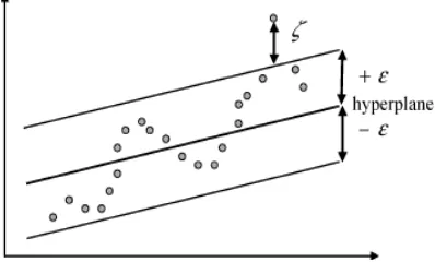
represent the solution to the above quadratic problem, making close to the predicted result phase target value .The non-zero value of the Lagrangian multiplier in the prediction in (7)which called the support vector in the prediction regression line. For all points in the tube, the Lagrangian multiplier is equal to zero does not help the regression function. Only meet (see Figure 1) the requirements as f x( ) y  , that the Lagrangian multiplier can be non-zero and used as support vector quantity.

The constant C introduced in (2) determines the penalty for the estimation error. A large C assigns higher penalties to false regression training to minimize errors and lower generalization, while a smaller C is allocated less that which allows edges to

i

(4)

[image:4.612.206.405.154.274.2]

Now, we have solved the Lagrangian multiplier of the W value. By applying the KKT condition we can calculate the variable b. In this case, it means that the Lagrange multiplier and the constraint must equal 0, ie:

Figure 1. SVR with radius ε matching tube data and positive slack variable measurement points lying outside the tub.

* *

( ( , ) ) 0 ( ( , ) ) 0

i i i i

y w x b y w x b

     

    

    

 

7

And,

(C _i) _i 0

 

8

* *

(C

 

_i) _i 0

 

9

Here i _and * i

 _{are slack variables. When} *

(0, )

i C

  _, *

, 0

i i

   _{, b can be}

calculated by:

*

( , ) (0, ) ( , ) (0, )

i i i

b y w x for C

 

   

   

 

10

(5)

MODEL APPLICATION

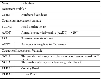
[image:5.612.180.418.246.363.2]

This paper analyzes the road traffic accident data of a certain section of Florida in the United States through R language programming. The number of traffic accidents is taken as the dependent variable, the length of the road segment, the traffic volume and the road surface condition are used as independent variables (model parameters are defined as Table II shows the support vector regression model. By sorting the importance of the independent variables, the two most important influencing factors, such as the length of the road segment and the traffic volume, are selected to re-establish the regression model.

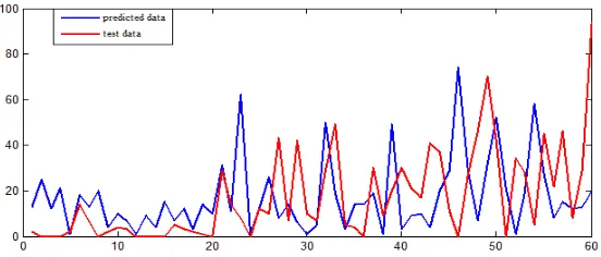
Figure 2. Comparison on prediction results of SVR linear kernel function and radial basis kernel function.

TABLE II. DEFINITION OF PARAMETERS IN THE MODEL. Name Definition

Dependent Variable

Count Number of accidents

Continuous independent variable

SLENG Road Section length

AADT Annual average daily traffic (AADT) × ×10−4

PSR Pavement condition score

AVGT Average car weight in traffic volume

Categorical Independent Variable

NOLA The number of single side lanes is less than or equal to 2 equal to 2

[image:5.612.134.461.428.684.2]

(6)

After using the random forest to determine the main influencing factors affecting the number of traffic accidents, 70% of the data is used as the training set, 30% of the data is used as the test set, and the SVR model is established. The main factors are used as the analysis features, and the linear kernel function is selected respectively. The radial basis kernel function performs support vector regression prediction to obtain the prediction result as shown in Fig. 2.

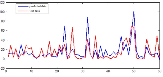
[image:6.612.167.445.289.417.2]

It can be seen from Fig. 2 that the fitting effect of the radial basis kernel function is better than that of the linear kernel function. To further verify the influence of all features on the number of traffic accidents and the impact of key features on the number of traffic accidents, Select the radial basis function with better fitting effect in the previous step as the kernel function, and perform regression prediction on the test data of all features and key features. The final prediction result is fitted as shown in the figure 3.

Figure 3. Comparison of prediction results of full features and key features of the kernel function Radial Kern.

[image:6.612.168.444.482.600.2]

(7)

[image:7.612.171.445.84.214.2]

Figure 5. SVR forecast results comparison chart.

SUMMARY AND PROSPECT

According to the above actual case analysis, the support vector model has a good predictive effect on the number of road traffic accidents. By comparison, for this practical problem, the support vector has better performance than the random forest. This is a comparison of the regression curves from the following figure. As can be seen:

Of course, the research in this paper also has some shortcomings. First, the data size of the problem is relatively small, and the data processing in the early stage is not very sufficient. In addition, this data does not involve missing and wrong, and it is relatively simple to handle.

In the future research, we should focus on the research of big data, improve the pre-processing of data, and pay attention to the processing of missing and missed data. Further enhance the prediction effect.

REFERENCES

1. Yixuan Sun, 2014, Analysis of Road Traffic Accidents Based on Data Mining [D]. Beijing: Beijing Jiaotong University,

2. Qian Zhou, Huapu Lu and Wei Xu The Law of Traffic Accidents and Its Model[J]. Journal of Traffic and Transportation Engineering, 2006, 6(4): 112-115.

3. C H Wu, J M Ho, D T Lee. Travel-time Prediction with Support Vector Regression[J]. IEEE Transactions on Intelligent Transportation Systems, 2004, 5(4):276-281.