A Method for Numerical Solution of Two Point Boundary Value Problems with Mixed Boundary Conditions

(1)

How to cite this paper: Pandey, P.K. (2014) A Method for Numerical Solution of Two Point Boundary Value Problems with Mixed Boundary Conditions. Open Access Library Journal, 1: e565.

http://dx.doi.org/10.4236/oalib.1100565

A Method for Numerical Solution of Two

Point Boundary Value Problems with

Mixed Boundary Conditions

Pramod Kumar Pandey

1,2

1_{Department of Mathematics, Dyal Singh College (Univ. of Delhi), New Delhi , India}

2_{Present Address: Department of Information Technology, College of Applied Sciences, Ministry of Higher} Education, Salalah, Sultanate of Oman

Email: [email protected]

Received 1 June 2014; revised 16 July 2014; accepted 26 August 2014

This work is licensed under the Creative Commons Attribution International License (CC BY).

http://creativecommons.org/licenses/by/4.0/

Abstract

In this article, we concerned with the development of a method for solving two point boundary value problems of ordinary differential equations. To develop method, we consider derivative of solution of a problem as an intermediate problem (IP). The analytical solution of the problem and IP were locally approximated by a nonlinear function with fixed step length. Some numerical ex-periments have been carried out to show the performance and effectiveness of the proposed thod. Also we obtained numerical value of derivative of solution as a byproduct of proposed me-thod. A clear conclusion can be drawn from the results that method converges with limited stabil-ity.

Keywords

Approximations, Boundary Value Problems, Fixed Step Size, Mixed Boundary Conditions, Maximum Absolute Error, Nonlinear Function, Stability

Subject Areas: Numerical Mathematics, Ordinary Differential Equation

1. Introduction

(2)

OALibJ | ODI:10.4236/oalib.1100565 2 September 2014 | Volume 1 | e565 two point boundary value problem with mixed boundary conditions. For such problem numerical methods are almost the only choice for getting solution.

Consider second order boundary value problems in ordinary differential equation of the form

( )2

_{( )}

₍

₎

_{[ ]}

_{( ) ( ) (}

₎

, , , , and , , , , .

y x = f x y y′ x∈ a b ⊂ y x y x′ f x y y′ ∈ (1)

subject to boundary conditions

( )

and ,

or and .

y a y b

α β

′ ′

= =

′ = ′ = (2)

where

(

α β, ′

)

and

(

α β′,

)

are real constants.

Generally, the existence and uniqueness conditions for the solution of two point boundary value problems can be different and difficult. Thus we use the specific assumption on f x y y′

(

, ,

)

to guarantee the existence and uniqueness for the solution of problem (1), those described in [1] [2]. We consider the presentation in this article as simple as possible. We shall not consider restrictions on source function f x y y′

(

, ,

)

for existence and uni-queness of the solution of the problem (1) those available in literature [3]. Thus the existence and uniuni-queness of the solution for the problem (1) is assumed. Further we assume that solution of the problem (1) depends conti-nuously on the given boundary conditions.

Numerical solution of problem (1), using finite difference method is an approximation to the value of solution of problem (1) at discrete points and depends on a step size, the distance between two successive discrete points. We use this idea to develop the proposed numerical method for the solution of the problem (1). The proposed method has the advantage of simplicity. The method is simple in sense that development of the method depends on the Taylor, Mac Lauren and exponential series expansion and seems to converge quadratically. But also we discuss the convergence of the approximate solution to the solution of the problem (1) in the limit of the step size go to zero. To the best of my knowledge, no similar method for the solution of problem (1) has been dis-cussed in literature so for.

We present in Section 2, the development and derivation of the numerical method for solving problem (1). Local truncation error and convergence is discussed in Section 3. The possibility of stability and computational performance of the method on model problems is discussed respectively in Sections 4 and 5. Conclusion and out view for future research are discussed in final Section 6.

2. Derivation of Method

We define the equal step size mesh points of the interval [a, b] as,

, 0,1, 2, , .

i

x = +a ih i=  N (3)

where x₀=a, x_N =b and h being step size and defined as h

(

b a

)

N

− = .

Let y_i, an approximate value of the theoretical solution y x

( )

of problem (1) at the mesh point x=x_i and

i

f an approximate value of source function f x y y′

(

_i, _i, _i

)

at the mesh point x=x_i. Further we assume that problem (1) posses unique solution in [a, b].

Suppose we have numerically solved the problem (1) up to the mesh point x_i and obtained numerical value

i

y , as an approximate value of y x

( )

, the solution of the problem (1) at mesh point at x=x_i. Let us assume local hypothesis [4] that y x

( )

_i = y_i. We are interested in obtaining y_i+₁, an approximate value of y x

( )

at

1

i x=x+ .

Further let we have y_i′+₁ an approximate value of IP, i.e. y x′

( )

, derivative of solution of the problem (1) at

the mesh point at x=x_i+₁ and assume that y x

( )

i+1 =yi′+1. We are interested in obtaining yi′, an approximate

value of y x′

( )

at the mesh point x=x_i.

Following the ideas in [5] [6], we propose an approximation to y x

(

_i+h

)

and y x′

( )

_i , the solution IP and derivative of solution of problem (1) respectively, as

(

)

( )

_{( )}

( )

(

)

( )

₍

₎

( )

2 2 0 2 0

e ,

e .

h

i i i i

h

i i i

y x h y x hy x a h y x

y x y x h b hy x h

ϕ θ

′

+ = + +

(3)

OALibJ | ODI:10.4236/oalib.1100565 3 September 2014 | Volume 1 | e565 where a b₀, ₀ are undetermined coefficients and ϕ

( ) ( )

h ,θ h are unknown differentiable functions of step length h.

From (4), let us define a function F h x y y y_i

(

, , , ′, ( )2

)

such that

( )

(

2

)

(

) ( )

( )

2 ( )2

_{( )}

( )

0

, , , , e h 0

i i i i i

F h x y y y′ ≡ y x +h −y x −hy x′ −a h y x ϕ = (5)

If we expand ϕ

( )

h in MacLauren series i.e.

( )

2

0 0

h h O h

ϕ =ϕ + ϕ′ + (6)

So, we have

( )

_{( )}

( )

2

eϕh = +1

ϕ

0 +h

ϕ

′ 0 +O h . (7)

If we expand y x

(

_i+h

)

in Taylor series about mesh point x=x_i in (5) and then using (7) in the expansion, we have

( )

(

2

)

2 ( )2

_{( )}

₍

_{( )}

₎

3 ( )3

_{( )}

( )2

_{( ) ( )}

0 0

1 1

, , , , 1 0 0 0.

2 6

i i i i

F h x y y y′ ≡h y x _ −a +ϕ _+h _ y x −a y x ϕ′ _=

    (8)

To determine a₀, ϕ

( )

0 and ϕ′

( )

0 , comparing coefficients of 2 h , 3

h both side in (8),we have

( )

(

)

0 1 1 0 2

a +ϕ =

( )

_{( )}( )

( )

[ ]

3 2 0 2 1

0 , 0 for any , .

6

i

i i

i

y x

a y x x a b

y x

ϕ′ = ≠ ∈

For simple expression and calculation, we assume ϕ

( )

0 =0, so we get

0 1 . 2 a =

( )

( )_{( )}

( )

3 2 1 0 . 3 i i y x y x

ϕ′ = (9)

Substituting value from (9) in (6), assuming the negligible contribution of the terms with O h

( )

2 , we have

( )

( )_{( )}

( )

3 2 , 3 i i y x h h y x

ϕ = (10)

Substituting values of a₀ and ϕ

( )

h from (9) and (10) in (4), we have

(

)

( )

_{( )}

( )_{( )} ( )_{( )} 3 2 2 3 2 e 2 i i y x h y x

i i i i

h

y x h y x hy x y x

 

 

 

′

+ = + + (11)

Following the similar steps as above, we can determine unknown coefficients in IP, second equation of (4). Thus we can write similar expression like (11) for IP as,

( )

(

)

( )

₍

₎

( )₍ ₎ ( )₍ ₎ 3 2 2 2 e i i

y x h h

y x h

i i i

y x y x h hy x h

 ₊ 

 

 ₊ 

 

′ = ′ + − + (12)

Thus, we can write our difference method for computation of solution and IP for problem (1) as,

(

)

( )

2 3

e 2 i i hf f

i i i i

h

y x h y x hy x f

′         ′ + = + +

( )

(

)

2 11

1e

i i

hf f

i i i

y x y x h hf

+ + ′         +

′ = ′ + − (13)

(4)

OALibJ | ODI:10.4236/oalib.1100565 4 September 2014 | Volume 1 | e565 d

d

i

f f y f

f f

x y x y

∂ ∂ ∂ 

′=_ + + _

′

∂ ∂ ∂

 

A difference method similar to (13), we can derive for other set of boundary conditions i.e. when y a′

( )

and

( )

y b are prescribed.

Thus we have developed an exponential single step method of the form

(

)

2

1 , , ,

2 i

i i i

h

y₊ = y +hy′+ G x y y′

(

)

1 1 , , i

i i

y′=y′₊ −hG x y y′ (14)

where G and G₁ are increment functions. The method (14) appears to me similar to the implicit Euler me-thod available in [7], for initial value problems in ordinary differential equation. But it is system of nonlinear equations in y_i+₁ and y′N i− +1, i=1, 2,,N and generally solved by iterative method. To solve this system of nonlinear equations, we have applied Newton Raphson iteration method. In variety of model second order boundary value problems reported in section 4,for computational purpose we have used single step finite differ-ence approximation in place of f_i′ i.e. hf_i′= f_i+₁− f_i.

3. The Local Truncation Error and Convergence

In this section, we consider the error associated to the proposed method (13). Let y x

( )

be the solution of problem (1) four times continuously differentiable in the domain [a, b]. Let the local truncation errors in solution and IP, derivative of solution of problem (1) are respectively T_i+₁ and DTi. So we define

( )

( ) ( )

( )

2 3 3 1 ₄ 1 1 2 1 3

2 , .

12

i

i i i i i i

i

y h

DT y x y y x x

y δ δ

+ + + +     ′

= − = _ − _ < <

   

(

)

3 6 , 6 i h

DT ≤ K+ M (15)

where M is Lipschitz constant for source function f x y y′

(

, ,

)

and K =maxx∈_{[ ]}a b_, y4

( )

x . Also,

(

)

1 1, 1, 2, 3, , ,

i i i

T₊ = y x +h −y₊ i=  N

(

) ( )

( )

( )_{( )} ( )_{( )} ( )

_{( )}

( )

3 2 2 3 1 2 4 4 4

1 1 1,

e 2 , 24 18 i i y x h y x

i i i i i

i i i

i i

h

T y x h y x hy x f

f

h h

hDT y x x

f δ δ         + + ′ = + − − − ′

= + − < <

(

)

3

1 15 88 .

6

i h

T+ ≤ K+ M (16)

Thus local truncation errors are bounded if 1 2 i

i f

f

′

< . It can be proved that increment functions G and G₁

satisfy Lipschitz condition. Also these functions are continuous in h. Therefore method (13) is convergent.

4. Stability Analysis

To discuss stability property of the method (13), we follow the same method as discussed in [8] [9]. Consider the Dahlquist test equation for stability,

( )2

_{( )}

2

_{( )}

_{[ ]}

, , and .

(5)

OALibJ | ODI:10.4236/oalib.1100565 5 September 2014 | Volume 1 | e565 subject to boundary conditions y a

( )

=y₀ and y a′

( )

=λy₀. Apply the method (13) to this test equation, we obtained a finite difference equation, assuming the negligible contribution of the terms with O h

( )

4 in the ex-pression,

( )

( ) ( )

_{( )}

2 2 2

3 1

2 3

e 1

2 2 3 18

1 , 1, 2, 3, , .

2 6

i i

h

i i i i i

i i

h h h h

y y hy y y hy y

h h

h y E h y i N

λ

λ λ λ λ

λ λ

+

 

′ ′  

= + + = + + + + +

 

 

 

 

= + + + + ≈ =

 

 



 

(17)

where the stability function E

( )

λh is some approximation to e .λh _{let define error equation}

( )

1 1 1

i+ = y xi+ −yi+



and substitute in (17), we have

( )

1

i+ =E λh i

  (18)

In some cases the numerical solution may differ considerably from the difference solution.The effect of local truncation error is bounded and E

( )

λh _i, is the propagation of the error from the previous step x_i to x_i+₁ in

computation of y x

( )

.

It will grow if E

( )

λh >1. Thus method is absolutely stable if E

( )

λh ≤1, so method (13) is absolutely stable if and only if −2.51275≤λh≤0. Similarly we can calculate propagation of the error from previous step

1

i

x+ to xi in IP, computation of y x′

( )

and is same as in y x

( )

.

5. Numerical Experiment

The results of numerical experiment will be presented in order to illustrate the performance of the proposed me-thod. We have shown in tables maximum absolute error computed on the discrete points in the interval of inte-gration for these experiments in their solution and derivative of solution, for different values of N. Let y_i and

i

y′ are the numbers calculated by (13) respectively which are an approximate value of the theoretical solution

( )

y x and IP, derivative of solution i.e. y x′

( )

at the point x=x_i. Maximum Absolute Error (MAE) is calcu-lated in both solution and derivative of solution by using formula

[ ],

( )

max , 2, 3, , 1 or 1, 2, , .

i

y i i

x a b

MAE y x y i N i N

∈

= − =  + = 

[ ],

( )

max , 1, 2, , , or 2, 3, , 1.

i

y i

x a b i

MAE′ = _∈ y x′ −y′ i=  N i=  N+

All computations in the examples consider were performed on MS Window 2007\professional operating sys-tem in the GNU FORTRAN environment version −99 compiler (2.95 of gcc) running on Intel Duo core 2.20 GHz PC. Both y x

( )

and y x′

( )

were computed on N nodes and iterations continued until either maximum difference between two iterates is less than 10−14 or number of iterations reached 103.

Problem 1.

Let us consider the following boundary value problem

( )2

_{( )}

( )

_{( )}

π π 2( )

_{( )}

e sin e ,

2 2

y x x x y x

y x = − y x + _ _ + f x

 

for x∈ =Ω

{

0≤ ≤x 1

}

,with the boundary conditions y x

( )

=1,y x′

( )

= −π 2,x∈ ∂Ω. In this example, the exact solution y x

( )

=cos

(

π 2x

)

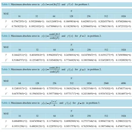
is known. We shall compute the MAE in the approximate solution y_i and the derivative of solution y′_j, at the mesh point i=2, 3,,N+1 and j=1, 2,,N for N=2p+1, p = 3, 4, ···, 9. We presented results in Table 1.

Problem 2.

( )2

_{( )}

sinh ,

y x =β βy +g x

(6)

OALibJ | ODI:10.4236/oalib.1100565 6 September 2014 | Volume 1 | e565

solution

( )

cosh

cosh x

y x β

β

= is known. We shall compute the MAE in the approximate solutiony_i and the de-

rivative of solution y′_j,at the mesh point i=1, 2, 3,,N and j=2, 3,,N+1 for N=2p+1,p=3, 4,, 9 and N =2p+1,p=5, 6,,11. We presented results in Table 2 and Table 3 for β =2 and β =5 respectively.

Problem 3.

( )2

_{( )}

cos ,

y x =βx y + f x

for x∈ =Ω

{

0≤ ≤x 1

}

,with the boundary conditions y x

( )

=0,y x′

( )

=0,x∈ ∂Ω. In this example, the exact

solution

( )

3 1

6 x

y x =β − is known. We shall compute the MAE in the approximate solution y_i and the

deriv-ative of solution y′_j, at the mesh point i=1, 2, 3,,N and j=2, 3,,N+1 for 1

2p , 3, 4, , 9.

N= + p= 

[image:6.595.82.538.269.726.2]

We presented results in Table 4 for β =10.

Table 1. Maximum absolute error in y x

( )

=cos

(

π 2x

)

and y x′

( )

for problem 1.

MAE

N

16 32 64 128 256 512 1024

y _{0.37967297(−2) 0.59528940(−3) 0.63126907(−4) 0.10699034(−4) 0.64298511(−5) 0.20265579(−5) 0.97602606(−6)} y′ 0.75638252(−2) 0.18921032(−2) 0.47309601(−3) 0.11825059(−3) 0.29586055(−4) 0.73965139(−5) 0.18725352(−5)

Table 2. Maximum absolute error in

( )

cosh

x

y x β

β

= and y x′

( )

for β=2 in problem 2.

MAE

N

16 32 64 128 256 512 1024

y _{0.16642511(−2) 0.40349363(−3) 0.99420547(−4) 0.24586916(−4) 0.63478947(−5) 0.16391277(−5) 0.74505806(−6)} y′ 0.51084757(−2) 0.12534857(−2) 0.31054020(−3) 0.77366829(−4) 0.18835068(−4) 0.52452087(−5) 0.11920929(−5)

( )

cosh

x

y x β

β

= and y x′

( )

for β=5 in problem 2.

MAE

N

64 128 256 512 1024 2048 4096

y _{0.12481017(−2) 0.30486844(−3) 0.75593591(−4) 0.18656254(−4) 0.50235540(−5) 0.17676502(−5) 0.47683716(−6)}

y′ 0.64787865(−2) 0.15945435(−2) 0.39577484(−3) 0.97751717(−4) 0.24318695(−4) 0.95367432(−5) 0.38146973(−5)

( )

3

1 6

x

y x =β − and y x′

( )

for β =10 in problem 3.

MAE

N

16 32 64 128 256 512 1024

(7)

OALibJ | ODI:10.4236/oalib.1100565 7 September 2014 | Volume 1 | e565

6. Conclusion

In this article, we have described a single step difference method of second order and applied to set of different

model problems with equal step length in range of 1 ,1 4096 16 h∈  _

 . The proposed method has advantages and

disadvantages when compared individually. The method based on exponential approximations, has good con-vergence in the computational domain. On the other hand very accurate iteration must be applied to solve nonli-near methods. As is evident from the results, method converges when we have applied Newton-Raphson method to solve system of nonlinear equations and gives O h

( )

2 accuracy. It is not clear how local assumption affect the overall solution of the problem. Investigation in this direction will be done in the future. Though stability discussed and heavily depends on approximation to exponential function and local assumption as well. In addi-tion, the development of this method will lead to possibility to approximate higher order derivatives in term of power of its lower order derivatives, to increase the order and accuracy of the method. Work in this specific di-rection is in progress. However our future works will also deal with similar extension of the present method to solve higher order boundary value problems.

References

[1] Aggarwal, R.P. (1986) Boundary Value Problems for Higher Order Differential Equations. World Scientific Publishing Co., Singapore. http://dx.doi.org/10.1142/0266

[2] Baxley, J.V. and Brown, E.S. (1981) Existence and Uniqueness for Two Point Boundary Value Problems. Proceedings of the Royal Society of Edinburgh Sect. A Mathematics, 88, 219-234.

[3] Copel, W.A. (1965) Stability and Asymptotic Behavior of Differential Equations. Heath Boston.

[4] Lambert, J.D. (1991) Numerical Methods for Ordinary Differential Systems. John Wiley, England.

[5] VanNiekerk, F.D. (1987) Non Linear One Step Methods for Initial Value Problems. Computers Mathematics with Ap-plications, 13, 367-371. http://dx.doi.org/10.1016/0898-1221(87)90004-6

[6] Pandey, P.K. (2013) Nonlinear Explicit Method for First Order Initial Value Problems. Acta Technica Jaurinensis, 6, 118-125.

[7] Butcher, J.C. (2008) Numerical Methods for Ordinary Differential Equations. 2nd Edition. John Wiley & Sons Ltd., Chichester. http://dx.doi.org/10.1002/9780470753767

[8] Jain, M.K., Iyenger, S.R.K. and Jain, R.K. (1987) Numerical Methods for Scientific and Engineering Computations

( )

2e . Wiley Eastern Ltd., New Delhi.

[9] Dahlquist, G. (1963) A Special Stability Problem for Linear Multistep Methods. BIT, 3, 27-43.