Damping Controller Based Quantum Particle Swarm Optimization for VSC HVDC to Improve Power System Stability

(1)

http://dx.doi.org/10.4236/epe.2014.612035

Damping Controller Based Quantum Particle

Swarm Optimization for VSC HVDC to

Improve Power System Stability

Naser Taheri

1

, Ahmad Hashemi

2

, Kowsar Kiani

3

1_{Islamic Azad University, Quchan Branch, Quchan, Iran}

2_{SAMA Technical and Vocational Training College, Islamic Azad University, Kermanshah Branch, Kermanshah, Iran} 3_{Department of Electrical Engineering, Semnan University, Semnan, Iran}

Email: [email protected], [email protected]

This work is licensed under the Creative Commons Attribution International License (CC BY).

http://creativecommons.org/licenses/by/4.0/

Abstract

The use of the supplementary controllers of a High Voltage Direct Current (HVDC) based on Vol-tage Source Converter (VSC) to damp low Frequency oscillations in a weakly connected system is surveyed. Also, singular value decomposition (SVD)-based approach is used to analyze and assess the controllability of the poorly damped electromechanical modes by VSC-HVDC different control channels. The problem of supplementary damping controller based VSC-HVDC system is formu-lated as an optimization problem according to the time domain-based objective function which is solved using quantum-behaved particle swarm optimization (QPSO). Individual designs of the HVDC controllers using QPSO method are evaluated. The effectiveness of the proposed controllers on damping low frequency oscillations is checked through eigenvalue analysis and non-linear time simulation under various disturbance conditions over a wide range of loading.

Keywords

VSC-HVDC, Power System Stability, Quantum Particle Swarm Optimization, Supplemetary Damping Controller

1. Introduction

(2)

electromechani-cal oscillations and transient stability are common problems that can happen in expanded power systems and transmit a large amount of power over long distance transmission lines [3] [4]. Increasing power system com-plexity gives rise to low frequency oscillations in the range of 0.2 - 3.0 Hz. If not well damped, these oscillations may keep growing in magnitude until loss of synchronism results [5]. In order to damp these power system os-cillations and increase system osos-cillations stability, the installation of power system stabilizer (PSS) is both economical and effective [5] [6]. However, PSSs may adversely affect voltage profile, result in leading power factor, and may not be able to suppress oscillations resulting from severe disturbances, especially those three-phase faults which may occur at the generator terminals [6]. Flexible AC transmission systems devices, such as Static VAR Compensators (SVC), Thyristor Control Series Compensators (TCSC), Static Synchronous Compensators (ST-ATCOM), and Unified Power Flow Controller (UPFC), are one of the recent propositions to alleviate such situations by controlling the power flow along the transmission lines and improving power oscil-lations damping [6][7]. Recently High Voltage Direct Current (HVDC) systems have greatly increased. They interconnect large power systems offering numerous technical and economic advantages. This interest results from practical characteristics and performance that include for example, nonsynchronous interconnection, con-trol of power flow and modulation to increase stability limits [8]. It is well known that HVDC may improve the transient and dynamic performance of the interconnected AC/DC system due to its fast electronic control of power flow also transient stability of the AC systems in a composite AC-DC system can be improved by taking advantage of the fast controllability of HVDC converters [6]-[10]. The conventional HVDC has several limita-tions and undesirable characteristics including being physically large and requiring the AC network with suffi-cient short-circuit ratio [11]-[13]. The Voltage Source Converter based on HVDC (VSC HVDC), which uses modern semiconductors with self-commuted ability, overcomes the disadvantages of conventional HVDC and is therefore more suitable for a weak AC network or a passive network without any power sources [13]. The con-trol of the voltage magnitude and the phase angle of the VSCs make the use of separate concon-trol for active and reactive power possible. The active power loop can be set to control either the active power or the dc-side vol-tage [14] [15]. A traditional lead-lag damping controller structure is preferred by the power system utilities be-cause of the ease of on-line tuning and also lack of assurance of the stability by some adaptive or variable struc-ture methods [7] [16] [17]. Having several local optimum parameters for a lead-lag controller, using of tradi-tional optimization approach is not suitable for such a problem. Thus, the heuristic methods as solution for find-ing global optimization are developed [18]-[20]. Particle swarm optimization (PSO) is a novel population based on metaheuristic, which utilizes the swarm intelligence generated by the cooperation and competition between the particle in a swarm and has emerged as a useful tool for engineering optimization [21]. This new approach features many advantages; it is simple, flexible, and fast and can be coded in few lines. Also, its storage re-quirement is minimal. However, the main disadvantage is that the PSO algorithm is not guaranteed to be glo-bally convergent. In order to overcome this drawback and improve optimization synthesis, in this paper, a quan-tum-behaved PSO technique is proposed for optimal tuning of HVDC based damping controller for enhancing of power systems low frequency oscillations damping. In this paper a novel approach is presented to model pa-rallel AC/DC power system namely Phillips-Heffron model based d-q algorithm in order to study dynamical stability of system. In addition, a block diagram representation is formed to analyze the system stability charac-teristics. Also, singular value decomposition (SVD) is used to choose damping control signal which has most effect on damping the electromechanical (EM) mode oscillations. A very powerful tool commonly used for this purpose is Popov-Belevitch-Hautus (PBH), which can be used to evaluate the EM mode controllability of the PSS and the different VSC HVDC controllers. A single machine infinite bus (SMIB) system equipped with a PSS and a VSC HVDC controller is used in this study. The problem of damping controllers design is formulated as an optimization problem to be solved using QPSO. The aim of the optimization is to search for the optimum controller parameter settings that maximize the minimum damping ratio of the system.

2. Problem Statement

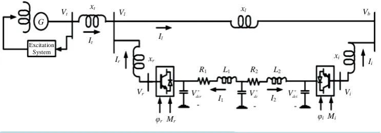
Figure 1 shows a SMIB system equipped with a VSC HVDC. As it can be seen the infinite bus is supplied by HVAC parallel connected with a VSC HVDC power transmission system. The VSC HVDC consists of two coupling transformer, two three-phase IGBT based voltage source converters (VSCs). These two converters are connected either back-to-back or joined by a DC cable, depending on the application.

(3)

Vt Vl xl

It Il

Ir xt

xi Vb

Vr

xr _I_i

I2 I1

Vi L2

L1

R1 R2

φr Mr φi Mi

dcr

V+ Vdc

[image:3.595.128.500.86.216.2]

+ dci V+ G Excitation System

Figure 1. A SMIB system Equationuipped with a VSC HVDC.

source converter behaves as a rectifier. It regulates the DC link voltage and maintains the magnitude of the vol-tage at the connected terminal. The second volvol-tage source converter acts as a controlled volvol-tage source, which controls power flow in VSC HVDC feeder. The four input control signals to the VSC HVDC are M PH Mr, r, i,

i

PH where M Mr, i are the amplitude modulation ratio and PH PHr, i are phase angle of the control signals

of each VSC respectively.

2.1. Power System Nonlinear Model

By applying Park’s transformation and neglecting the resistance and transients of the coupling transformers, the VSC HVDC can be modeled:

( )

cos 0 ₂ 0 sin 2

r dcr r

ld r rd

lq r lrq r dcr r

M V

V x I

V x I M V

ϕ ϕ          _ _ = +   ₋   _ _           (1)

( )

cos 0 ₂ 0 sin 2

i dci i

bd i id

bq i iq i dci i

M V

V x I

V x I M V

ϕ ϕ          _ _ = +   ₋   _ _           (2)

(

1 2

)

dc

CV = − I +I (3)

1

1 1 1

d

d dc dcr

I

L V V R I

t = − − (4)

2

2 2 2

d

d dc dci

I

L V V R I

t = − − (5)

where V V Il, b, r and Ii are the middle bus voltage, infinite bus voltage, flowed current to rectifier and inverter

respectively. C And V_dc are the DC link capacitance and voltage, respectively. C C Vr, i, dcr and Vdci are the

DC capacitances and voltages of rectifier and inverter respectively. The non-linear model of the SMIB system of Figure 1is:

(

1

)

b

δ ω ω

= − (6)

(

Pm Pe D

)

M ω

ω= − − (7)

(

)

(

fd d d t q

)

q

do

E x x I E

E T ′ ′ − − − ′ = ′

(4)

(

)

(

A ref t PSS fd

)

fd

A

K V V u E

E

T

− + − =

 (9)

where: P_e=V I_{td td} +V I_{tq tq}, V_t = V_td2+V_tq2, V_td =x I_{q tq}, V_tq =E_q′−x I′_{d td}, I_td =I_ld −I_rd, I_tq =I_lq−I_rq where

m

P and P_e are the input and output power , respectively; M and D the inertia constant and damping coefficient , respectively; ω_b the synchronous speed;

δ

and ω the rotor angle and speed, respectively;

,

q fd

E E′ and V_t the generator internal, field and terminal voltages, respectively; T_do′ the open circuit field time constant; x xd, d′ and xq the d-axis, d-axis transient reactance, and q-axis reactance, respectively; KA

and T_A the exciter gain and time constant, respectively; V_ref the reference voltage. Also, from Figure 1we have:

t t t l

V = jx I +V (10)

t t t l l b

V = jx I + jx I +V (11)

t t t r l t

r

V jx I V I I

jx

− −

= − (12)

where I_t, V_r, I_l and V_b are the armature current, rectifier voltage, infinite bus current and voltage respec-tively. From Equations (10)-(12) we can have:

( )

cos sin

2 l r

dcr r b

r tq q x M V V x I Zx A

ϕ + δ

=

+ (13)

( )

sin cos

2

l r

q dcr r b

r td

d

x M

ZE V V

x I Zx A ϕ δ ′ − − =

′ + (14)

And for inverter side:

( )

cos sin

2

i

b dci i

id i M V V I x δ ϕ − +

= (15)

( )

sin cos

2

i

b dci i

iq i M V V I x

δ − ϕ

= (16)

2.2. Power System Linearized Model

By linearizing Equations (1)-(7) (13)-(16):

b

δ ω ω

∆ = ∆ (17)

(

Pm Pe D

)

M ω ω ∆ − ∆ − ∆

∆ = (18)

(

)

(

)

'

fd d d td q

q

do

E x x I E

E

T

′ ′

∆ − − ∆ − ∆

′

∆ = (19)

(

)

(

A t PSS fd

)

fd

A

K V u E

E

T

∆ + ∆ − ∆

∆ = (20)

(5)

5 6 _r

t q vdcr dcr vM r v r r

V K δ K E′ K V K M K_φ ϕ

∆ = ∆ + ∆ + ∆ + ∆ + ∆ (21)

1 2

e q pdcr dc pMr r p r r

P K

δ

K E′ K V K M K ϕ

ϕ

∆ = ∆ + ∆ + ∆ + ∆ + ∆ (22)

3 4

q q q r r qMr r qdcr dcr

E K E′ K

δ

K_ϕ

ϕ

K M K V

∆ = ∆ + ∆ + ∆ + ∆ + ∆ (23)

31 32 33 34 35

1 1

dcr q dcr r r

r r r r r r

C C C C C

V E V I M

C δ C ′ C C C C ϕ

∆ = ∆ + ∆ + ∆ + ∆ + ∆ + ∆ (24)

Substitute Equations (21)-(23) in (17)-(20) we can obtain the state variable of the power system installed with the VSC HVDC to be (state space model):

X =AX+BU and

1 2

, , _q, _fd, _dcr, _I , _dc, , _dci T

X = ∆ ∆ ∆_

δ ω

E′ ∆E ∆V ∆ ∆V ∆ ∆I V _ (25)

[

]

T

, , , ,

r r i i PSS

U = ∆M ∆ϕ ∆M ∆ϕ u

where ∆Mi,∆Mr,∆ϕi,∆ϕr and uPSS are the linearization of the input control signals of the VSC HVDC and

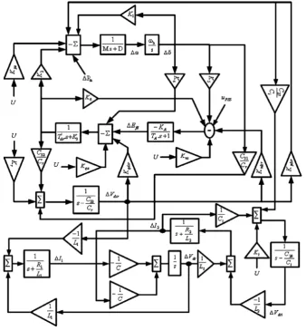
[image:5.595.144.483.344.710.2]

PSS output respectively. The linearized dynamic model of Equation (25) can be shown by Figure 2. In this fig-ure Kpu,Kqu,Kvu,Kr and Ki are defined:

(6)

1 2

3 4

5 6

31 32 33

1

1 1 1

2

2 2 2

27 28

0 0 0 0 0 0 0 0

0 0 0 0 0

1

0 0 0 0 0

1

0 0 0 0 0

1

0 0 0 0 0

1 1

0 0 0 0 0 0

1 1

0 0 0 0 0 0 0

1 1

0 0 0 0 0 0

1

0 0 0 0 0 0

pdcr

qdcr

do do do do

A A A vdcr

A A A A

r r r r

i i i

b

K

K D K

M M M M

K K

K

T T T T

K K K K K K

T T T T

C C C

A C C C C

R

L L L

C C

R

L L L

C C

C C C

ω    − − − −   − − − ′ ′ ′ ′ − − − − = − − − − − − −                                                34 35 29 30

0 0 0 0 0

0 0 0

0 0

0 0 0

0 0 0 0 0

0 0 0

pMr p r

qMr q r

do do

v r A

vMr A A

A A A

r r i i K K M M K K T T K K

K K K

T T T

B C C C C C C C C ϕ ϕ ϕ      ₋ ₋       ₋ ₋   ′ ′    ₋ ₋      =                      

34 35 29 30

, , 0, 0, 0 , , , 0, 0, 0 , , , 0, 0, 0

, , 0, 0, 0 , 0, 0, , , 0

pu pMr p r qu qMr q r vu vMr v r

r i

r r i i

K K K K K K K K K

C C C C

K K

C C C C

ϕ ϕ ϕ

      =_ _ =_ _ _{= } _     =_ _ _{= } _    

It can be seen that the configuration of the Phillips-Heffron model is exactly the same as that installed with SVC, TCSC, TCPS, UPFC and STATCOM. Also from Equation (25) it can be seen that there five choice of in-put control signals of the VSC HVDC to superimpose on the damping function of the VSC HVDC

, , ,

i r i r

M M ϕ ϕ

∆ ∆ ∆ ∆ and u_PSS. Therefore, in designing the damping controller of the VSC HVDC, besides set-ting its parameters, the selection of the input control signal of the VSC HVDC to superimpose on the damping function of the VSC HVDC is also important.

3. PSO versus QPSO

(7)

candidate, called a “particle”, flies in the problem space (similar to the search process for food of a bird swarm) looking for the optimal position. A particle with time adjusts its position to its own experience, while adjusting to the experience of neighboring particles. If a particle discovers a promising new solution, all the other particles will move closer to it, exploring the region more thoroughly in the process.

PSO starts [22] with a population of random solutions “particles” in a D-dimension space. The ith particle is

represented by X_i =

(

x_i₁,x_i₂,,x_iD

)

. Each particle keeps track of its coordinates in hyperspace, which are asso-ciated with the fittest solution it has achieved so far. The value of the fitness for particle i (pbest) is also stored as P_i=

(

p_i₁,p_i₂,,p_iD

)

. The global version of the PSO keeps track of the overall best value (gbest), and its location, obtained thus far by any particle in the population [21] [22]. PSO consists of, at each step, changing the velocity of each particle toward its pbest and gbest according to following Equations:

( ) (

)

( )

(

)

1 2

id id id id gd id

v = ×w v +C ×rand × p −x +C ×rand × p −x (26)

id id id

x =x +v (27)

where, p_id = pbest and p_gd = gbest PSO algorithm is as follow:

Step 1: Initialize an array of particles with random positions and their associated velocities to satisfy the in-equality constraints.

Step 2: Check for the satisfaction of the equality constraints and modify the solution if required. Step 3: Evaluate the fitness function of each particle.

Step 4: Compare the current value of the fitness function with the particles’ previous best value (pbest). If the current fitness value is less, then assign the current fitness value to pbest and assign the current coordinates (po-sitions) to pbest.

Step 5: Determine the current global minimum fitness value among the current positions.

Step 6: Compare the current global minimum with the previous global minimum (gbest). If the current global minimum is better than gbest, then assign the current global minimum to gbest and assign the current coordi-nates (positions) to gbest.

Step 7: Change the velocities according to Equation (26).

Step 8: Move each particle to the new position according to Equation (27) and return to Step 2.

Step 9: Repeat Step 2 - 8 until a stopping criterion is satisfied or the maximum number of iterations is reached. The main disadvantage is that the PSO algorithm is not guaranteed to be global convergent [24]. The dynamic behavior of the particle is widely divergent forming that of that the particle in the PSO systems in that the exact values of x_i and v_i cannot be determined simultaneously. In quantum world, the term trajectory is meaning-less, because x_i and v_i of a particle cannot be determined simultaneously according to uncertainty principle. Therefore, if individual particles in a PSO system have quantum behavior, the PSO algorithm is bound to work in a different fashion. In the quantum model of a PSO called here QPSO, the state of a particle is depicted by wave function W(x, t) instead of position and velocity [23] [24]. Employing the Monte Carlo method, the par-ticles move according to the following iterative equation:

1

Ln , 0.5

1

Ln , 0.5

i i i

x p Mbest x k

u

x p Mbest x k

u

β

 

= + ⋅ − _{ } ≤

   

= − ⋅ − _{ } >

 

(28)

where u and k are values generated according to a uniform probability distribution in range [24], the para-meter β is called contraction expansion coefficient, which can be tuned to control the convergence speed of the particle. In the QPSO, the parameter β must be set as β <1.782 to guarantee convergence of the particle

[23]. Where Mbest called mean best position is defined as the mean of the pbest positions of all particles, i.e.:

1

1 N i d

Mbest P

N =

=

∑

. (29)

(8)

Step 1: Initialization of swarm positions: Initialize a population (array) of particles with random positions in the n-dimensional problem space using a uniform probability distribution function.

Step 2: Evaluation of particle’s fitness: Evaluate the fitness value of each particle.

Step 3: Comparison to pbest (personal best): Compare each particle’s fitness with the particle’s pbest. If the current value is better than pbest, then set the pbest value equal to the current value and the pbest location equal to the current location in n-dimensional space.

Step 4: Comparison to gbest (global best): Compare the fitness with the population’s overall previous best. If the current value is better than gbest, then reset gbest to the current particle’s array index and value.

Step 5: Updating of global point: Calculate the Mbest using Equation (29).

Step 6: Updating of particles’ position: Change the position of the particles according to Equation (28), where c1 and c2 are two random numbers generated using a uniform probability distribution in the range [0, 1].

Step 7: Repeating the evolutionary cycle: Loop to Step 2 until a stop criterion is met, usually a sufficiently good

3.1. PSS and VSC-HVDC Damping Controller

3 1

2 4

1 1

1 1 1

w pss

w

sT sT sT

u k

sT sT sT ω

 +  + 

= _ _ _∆

+ _ + _ + _ (30)

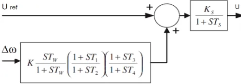
The VSC-HVDC damping controllers are of the structure shown in Figure 3 which u can be ∆Mi,∆Mr, ,

i r

ϕ ϕ

∆ ∆ . However, an electrical torque in-phase with the speed deviation is to be produced in order to enhance damping of the system oscillations. It includes gain block, signal-washout block and lead-lag compensator. The parameters of the damping controller are obtained using QPSO algorithm.

VSC-HVDC Controller Design Using QPSO

To obtain optimal parameters, this paper employs QPSO [24] to enhance optimization synthesis and find the global optimum value of fitness function. The objective function (which must be minimized) is defined as fol-lows [25]:

1 0

d

t N

i j

f t ω t

=

∑∫

∆ (31)

where t is the time range of simulation and N is the total number of operating points for which the optimi-zation is carried out. The design problem can be formulated as the following constrained optimioptimi-zation problem, where the constraints are the controller parameters bounds [22]:

min max min max min max min max

min max 1 1 1 2 2 2 3 3 3 4 4 4

Minimize :

Subject : , , , ,

f

K ≤K≤K T ≤ ≤T T T ≤T ≤T T ≤T ≤T T ≤T ≤T (32)

Typical ranges of the optimized parameters are [0.01 - 100] for K and [0.01 - 1] for T₁, T₂, T₃ and T₄. The proposed approach employs QPSO algorithm to solve this optimization problem and search for an optimal or near optimal set of controller parameters.

3.2. Controllability Measurement Based on SVD

[image:8.595.186.435.619.706.2]

Controllability shows how the state variables describing the behavior of a system can be influenced by its inputs.

(9)

More accurately, the dynamical system x=Ax+Bu or the pair (A, B) is said to be state controllable if, for any initial state x

( )

0 =x₀ any time t₁>0 and any final state x₁ there exist an input u(t) such that x t

( )

₁ =x₁. Otherwise the system is said to be state uncontrollable.

In damping of power oscillations, it is necessary to determine controllability for specific eigenvalues (elec-tromechanical mode). A very powerful tool commonly used for this purpose is Popov-Belevitch-Hautus (PBH) test which is described as below. It includes in evaluating the rank of matrices:

( )

_k

[

_k , _i

]

C λ = λ I−A b (33)

which λ_k is the kth eigenvalue of the matrix A, I is the identity matrix, b_i is the column of B corresponding to ith input ui. The mode λk of linear system in state space form is controllable if matrix C

( )

λk has full row rank. The rank of matrices C

( )

λ_k can be evaluated by their singular values. The singular values are defined as below:

If G is a m n× complex matrix, then there exist unitary matrices U and V with dimensions of m m×

and n n× , respectively, such that:

H

G= ΣU V (34)

where 1 0

0 0

Σ

 

Σ =  

 , Σ =1 diag

(

σ1,,σr

)

With σ₁≥≥σr ≥0 where r=min

{ }

m n, and σ1,,σr are the singular values of G.

The minimum singular value σ_r represents the distance of the matrix G from all the matrices with a rank of r−1 [26]. This property can be used to quantify modal controllability and observability [26]. The matrix H (and J) can be written as H=

[

h h h h_{1 2 3 4}

]

where h_i is a column vector corresponding to the ith input. The minimum singular value, σ_min of the matrix

[

λI−A h, _i

]

indicates the capability of the ith input to control the mode associated with the eigenvalue

λ

. Actually, the higher σ_min, the higher the controllability of this mode by the input considered. As such, the controllability of the EM mode can be examined with all inputs in order to identify the most effective one to control the mode. Thus, the choice of input through the PBH test is done by selecting those with the largest of the minimum singular values of matrix C

( )

λ_k .

4. Simulation Results

Power system information is given in Appendix A. Constant coefficients in modeling are calculated according information which given in appendix B. In this paper, we consider ∆

ω

(rotor speed deviation) as outputs and five inputs which are Mr,

ϕ

r,Mi,

ϕ

i,upss i.e. modulation index, phase angle of rectifier and inverter

respec-tively and finally PSS input. Selecting an affective coupling between inputs-output for damping oscillation of the power system is one of the most important goals of this paper. Following section consider this topic.

4.1. Controllability Measure by Using PBH Test

SVD based on PBH is employed to measure the controllability of the electromechanical mode (EM) mode from each of the five inputs: Mr,

ϕ

r,Mi,

ϕ

i,upss. The minimum singular value σmin is estimated over a wide range

of operating conditions. For SVD analysis, P_e ranges from 0.01 to 1.5 Pu and Q_e= −

[

0.4, 0, 0.4

]

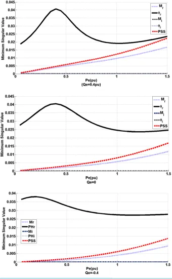
. At each loading condition, the system model is linearized, the EM mode is identified, and the SVD-based controllability and observability measure is implemented. For comparison purposes, the minimum singular value for all inputs at Qe = −0.4, 0 and 0.4 Pu is shown in Figure 4, respectively. From these figures, the following can be noticed:

• EM mode controllability via ϕ_r is always higher than that of any other input.

• The capabilities of

ϕ

r,M ur, pss to control the EM mode is higher than that of Mi,ϕi.

• All control signals have low EM mode controllability in low load condition except ϕ_r.

According to what said above, to design supplementary controller based VSC-HVDC, applying damping sig-nal to ϕ_r can have most affection on oscillation mode.

4.2. Using QPSO to Obtain Parameters of Supplementary Controllers

(10)

[image:10.595.143.484.87.639.2]

Figure 4. Minimum singular value for different value for Qe.

that the objective function is optimized. The final parameters are given inTable 1.

(11)

[image:11.595.83.545.81.725.2]

Table 1. Parameters of supplementary controller designed by QPSO.

PSS Mr ϕr Mi ϕi

k −0.3572 3.3498 −60.088 95 77.509

1

T 0.72 3.4 0.045 0.47 0.84

2

T 0.15 0.027 0.053 0.04 1.8

3

T 5.6 8.2 0.1 4.1 12

4

T 0.26 1.1 0.073 0.33 4.1

Table 2. Synchronous machine condition.

t V e

Q e

P

Operating Condition

1 0.015

1 1

λ (Nominal) Linearized system

1 0.4

1.2 2

λ (Heavy) Linearized system

1 0.015

1 3

λ (Nominal) Nonlinear system

1 0.4

1.2 4

λ (Heavy) Nonlinear system

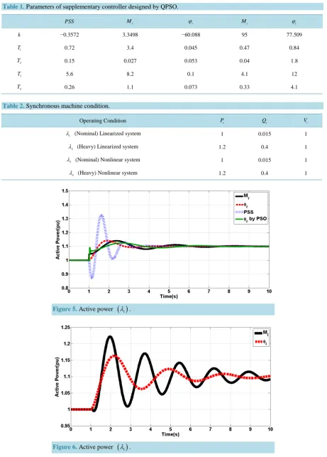
Figure 5. Active power

( )

λ1 .

(12)

Parameters of PSO based damping controller are as: k= −98.021,T₁=0.12,T₂=0.223,T₃=3.2,T₄=0.27 Testing model consists of small changing in mechanical power

(

∆P_m=0.1

)

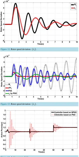
which is applied at t=1 s. Test-ing nonlinear model includes small changTest-ing in mechanical power

(

∆P_m=0.1

)

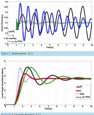
at t=25 s and three phase fault at infinite bus at time t=75 s that is removed after 7 cycles. Figures 5-13show the linear power system response in condition λ₁ and λ₂. Because of results which obtained by SVD analysis and also system re-sponse for λ₁ condition, in λ₂ we just used from rectifier and PSS inputs for applying damping signal and

,

i i

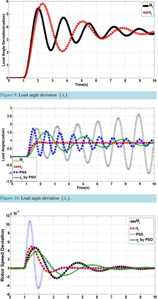
M ϕ are omitted. According to these figures, damping controller based on QPSO damps active power, rotor speed oscillations and load angle better than PSO-based compensator for loading condition. Also, using of ϕ_r can guarantee best damping results. Figures 14-19show the nonlinear power responses. According to these fig-ures, QPSO based damping controller applying to ϕ_r damps active power, terminal voltage and rotor speed oscillations better than PSO.

5. Conclusion

In this paper, SVD has been employed to evaluate the electromechanical mode controllability to PSS and the four VSC HVDC control signals. It has been shown that the electromechanical mode is most powerfully con-trolled via a wide range of loading conditions. Also, the quantum-behaved particle swarm optimization algo-rithm has been successfully applied to the robust design of VSC HVDC based damping controllers. The effec-tiveness of the proposed VSC HVDC controllers for improving transient stability performance of a power sys-tem are demonstrated by a weakly connected power syssys-tem subjected to different severe disturbances. The

[image:12.595.155.472.328.714.2]

Figure 7. Active power

( )

λ2 .

(13)

Figure9. Load angle deviation

( )

λ1 .

Figure 10. Load angle deviation

( )

λ2 .

[image:13.595.157.472.89.686.2] [image:13.595.156.471.446.709.2]

(14)

[image:14.595.156.473.89.712.2]

Figure12.Rotor speed deviation

( )

λ₁ .

Figure 13. Rotor speed deviation

( )

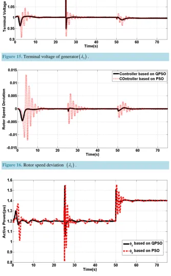
λ₂ .

[image:14.595.158.468.95.279.2]

(15)

[image:15.595.151.477.87.267.2]

Figure 15.Terminal voltage of generator

( )

λ₃ .

Figure 16. Rotor speed deviation

( )

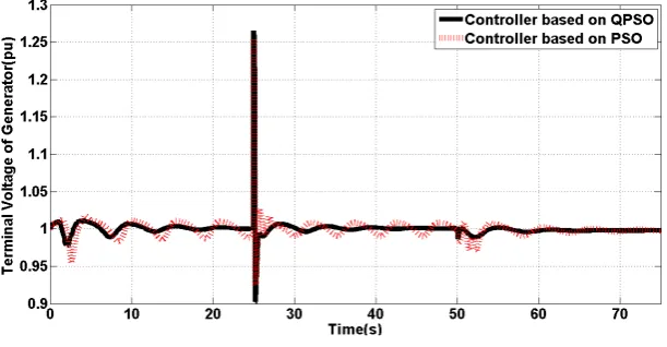
λ3 .

[image:15.595.146.481.167.706.2]

(16)

[image:16.595.161.467.89.248.2] [image:16.595.161.471.279.478.2]

Figure 18.Terminal voltage of generator

( )

λ₄ .

Figure 19.Rotor speed deviation

( )

λ4 .

non-linear time-domain simulation results show the effectiveness of the proposed controller and their ability to provide good damping of low frequency oscillations.

References

[1] Hsu, Y.-Y. and Wang, L. (1988) Damping of a Parallel Ac-Dc Power System Using Pid Power System Stabilizers and Rectifier Current Regulators. IEEE Transactions on Energy Conversion, 3, 540-547. http://dx.doi.org/10.1109/60.8065

[2] Flourentzou, N., Agelidis, V.G. and Demetriades, G.D. (2009) VSC-Based HVDC Power Transmission Systems: An Overview. IEEE Transactions onPower Electron, 24, 592-602. http://dx.doi.org/10.1109/TPEL.2008.2008441

[3] Zhang, L., Harnefors, L. and Peter, H. (2011) Interconnection of Two Very Weak AC Systems by VSC-HVDC Links Using Power-Synchronization Control. IEEE Transactions on Power Systems, 26,344-355.

[4] Licéaga-Castro, E., Licéaga-Castro, J. and Ugalde-Loo, C.E. (2005) Beyond the Existence of Diagonal Controllers: From the Relative Gain Array to the Multivariable Structure Function. Proceedings of the 44th IEEE Conference on Decision and Control and 2005 European Control Conference, 7150-7156.

[5] Shayeghi, H., Shayanfar, H.A., Jalilzadeh, S. and Safari, A. (2009) A PSO Based Unified Power Flow Controller for Damping of Power System Oscillations. Energy Conversion and Management, 50, 2583-2592.

http://dx.doi.org/10.1016/j.enconman.2009.06.009

[6] Banaei, M. and Taheri, N. (2001) An Adaptive Neural Damping Controller for HVDC Transmission Systems. Euro-pean Transactions on Electrical Power, 21, 910-923. http://dx.doi.org/10.1002/etep.485

(17)

PSO in Multi-Machine Power System. Energy Conversion and Management, 51, 2930-2937.

[8] Latorre, H.F. and Ghandhari, M. (2011) Improvement of Power System Stability by Using a VSC-HVDC. Electrical Power and Energy Systems, 33, 332-339. http://dx.doi.org/10.1016/j.ijepes.2010.08.030

[9] Bahrman, M.P. and Johnson, B.K. (2007) The ABCs of HVDC Transmission Technologies. IEEE Power & Energy, 5, 34-35, 44.

[10] Kundur, P. (1994) Power System Stability and Control. McGraw-Hill, New York.

[11] Guo, C.Y. and Zhao, C.Y. (2010) Supply of an Entirely Passive AC Network through a Double-Infeed HVDC System.

IEEE Transactions on Power Electronics, 25, 2835-2841. http://dx.doi.org/10.1109/TPEL.2010.2050214

[12] Han, B.M., Baek, S.T., Bae, B.Y. and Choi, J.Y. (2006) Back-to-Back HVDC System Using a 36-Step VoltageSource Converter. IEE Proceedings-Generation, Transmission and Distribution, 153, 677-683.

http://dx.doi.org/10.1049/ip-gtd:20060053

[13] Tang, X. and Lu, D. (2014) Enhancement of Voltage Quality in a Passive Network Supplied by a VSC-HVDC Trans-mission under Disturbances. International Journal of Electrical Power & Energy Systems, 54, 45-54.

http://dx.doi.org/10.1016/j.ijepes.2013.06.030

[14] Du, C.Q., Bollen, M.H.J.,Agneholm, E. and Sannino, A. (2007) A New Control Strategy of a VSC-HVDC System for High-Quality Supply of Industrial Plants. IEEE Transactions on Power Delivery, 22, 2386-2394.

http://dx.doi.org/10.1109/TPWRD.2007.899622

[15] Du, C., Agneholm, E. and Olsson, G. (2008) Comparison of Different Frequency Controllers for a VSC-HVDC Sup-plied System. IEEE Transactions on Power Delivery, 23, 2224-2232. http://dx.doi.org/10.1109/TPWRD.2008.921130

[16] Panda, S. and Prasad Padhy, N. (2008) Comparison of Particle Swarm Optimization and Genetic Algorithm for FACTS Based Controller Design. Applied Soft Computing, 8, 1418-1427. http://dx.doi.org/10.1016/j.asoc.2007.10.009

[17] Shayeghi, H., Shayanfar, H.A., Jalilzadeh, S. and Safari, A. (2009) A PSO Based Unified Power Flow Controller for Damping of Power System Oscillations. Energy Conversion and Management, 50, 2583-2592.

[18] Panda, S., Swain, S.C., Rautray, P.K., Malik, R. and Panda, G. (2010) Design and Analysis of SSSC-Based Supple-mentary Damping Controller. Simulation Modelling Practice and Theory, 18, 1199-1213.

http://dx.doi.org/10.1016/j.simpat.2010.04.007

[19] Panda, S. (2011) Differential Evolution Algorithm for SSSC-Based Damping Controller Design Considering Time De-lay. Journal of the Franklin Institute, 348, 1903-1926. http://dx.doi.org/10.1016/j.jfranklin.2011.05.011

[20] Panda, S. (2009) Multi-Objective Non-Dominated Shorting Genetic Algorithm-II for Excitation and TCSC-Based Controller Design. Journal of Electrical Engineering, 60, 87-94.

[21] Shayeghi, H., Jalili, A. and Shayanfar, H.A. (2008) Multi-Stage Fuzzy Load Frequency Control Using PSO. Energy Conversion and Management, 49, 2570-2580. http://dx.doi.org/10.1016/j.enconman.2008.05.015

[22] Awami, A., Abdel-Magid, Y. and Abido, M.A. (2007) A Particle-Swarm-Based Approach of Power System Stability Enhancement with Unified Power Flow Controller. International Journal of Electrical Power & Energy Systems, 29, 251-259. http://dx.doi.org/10.1016/j.ijepes.2006.07.006

[23] Shayeghi, H., Shayanfar, H.A., Jalilzadeh, S. and Safari, A. (2010) Tuning of Damping Controller for UPFC Using Quantum Particle Swarm Optimizer. Energy Conversion and Management, 51, 2299-2306.

[24] Coelho, L.S. (2008) A Quantum Particle Swarm Optimizer with Chaotic Mutation Operator. Chaos, Solitons & Frac-tals, 37, 1409-1418. http://dx.doi.org/10.1016/j.chaos.2006.10.028

[25] Shayeghi, H., Shayanfar, H.A. and Jalili, A. (2006) Multi Stage Fuzzy PID Power System Automatic Generation Con-troller in Deregulated Environments. Energy Conversion and Management, 47, 2829-2845.

(18)

Appendix

The test system parameters are (all in pu): Machine and Exciter:

1, 0.6, 0.3, 0, 8, 5.044, 60, 1, 120, 0.015

d q d do ref A A

x = x = x′ = D= M = T′ = freq= v = K = T =

Transmission line and transformer reactance: xt =0.1,xl =1,xr =xi =0.15 VSC HVDC: Vdcr =2,Vdci =1.95,Cr =Ci =2,L₁=L₂=0.09,C=0.09 Coefficients are: 1 l r x Z x

= + , t

t l

r

x

A x x

x

= + + ,

[ ]

A = +A Zx′_d,

[ ]

B = +A Zx_q

( )

[ ]

1 cos b V C B δ = ,

( )

[ ]

2 sin 2

l r dc r r

x M V C x B ϕ = − ,

( )

[ ]

3 cos 2

l dc r r x V C x B ϕ = ,

( )

[ ]

4 cos 2

l r r

r x M C x B ϕ = , 5 Z C A = ,

( )

[ ]

6 sin b V C A δ = ,

( )

[ ]

7 cos 2

l r dc r r

x M V C

x A ϕ

= − , C_a =

(

x_q−x_d′

)

I_t,

( )

[ ]

8

sin 2

l dc r r x V C x A ϕ = − ,

( )

[ ]

9 cos 2

l r dc r r

x M V C

X A ϕ

= − , C_b =E_q′+

(

x_q−x_d′

)

, K₁=C C_b ₁+C C_a ₆,

(

)

(

)

2 t 1 q d 5

K =I + x −x′ C , K_pdcr =C C_b ₄+C C_a ₉, K_pMr =C C_b ₃+C C_a ₈, K_pPHr =C C_b ₂+C C_a ₇,

d d

x −x′ =J, K₃ = +1 JC₅, K₄=JC₆, K_{q r}_ϕ =JC₇, K_qMr =JC₈, K_qdcr =JC₉,

1

t

L V

= , K₅ =L V x C

(

_td _q ₁−V x C_tq _d′ ₆

)

, K₆=LV_tq

(

1−x C_d′ ₅

)

, K_Vdcr =L V x C

(

_td _q ₄−V x C_tq _d′ ₉

)

,

(

3 8

)

VMr td q tq d

K =L V x C −V x C′ , K_{V r}ϕ =L V x C

(

_td _q ₂−V x C_tq _d′ ₇

)

, d t

r

x x

E x ′ +

= , q t

r x x F x + = , 10 5 1 r C EC x

= − , C₁₁=EC₆, ₁₂ ₇ sin

( )

2 r

dcr r

r

M

C EC V

x ϕ

= − , ₁₃ 1 cos

( )

₈

2 _r r r

C M EC

x ϕ = + ,

( )

14 9 1 cos

2 _r r

C EC

x ϕ

= + , C₁₅ =FC₁, ₁₆ 1 sin

( )

₂

2 _r dcr r

C V FC

x ϕ

= + , ₁₇ 1 cos

( )

₄

2 _r r r

C M FC

x ϕ = − + ,

( )

18 3 1 cos

2 _r dcr r

C FC V

x ϕ

= − , ₁₉ 1 _bd

i

C V

x

= , ₂₀ 1 sin

( )

2 _i i i

C M

x ϕ

= , ₂₁ 1 sin

( )

2 _i dcr i

C V x ϕ = ,

( )

22 1 cos

2 _i i dci i

C M V

x ϕ

= , ₂₃ 1 _bq

i

C V

x

= , ₂₄ 1 cos

( )

2 _i i i

C M

x ϕ

= − , ₂₅ 1 cos

( )

2 _i dci i

C V x ϕ = − ,

( )

26 1 sin

2 _i dci i

C V

x ϕ

= , f₁ =_0.5 cos

( )

ϕ_i I_id+0.5sin

( )

ϕ_i I_iq_, f₂= − −_ 0.5sin

( )

ϕ_i I_id+0.5 cos

( )

ϕ_i I_iq_,

( )

3 0.5 icos i

f = − M ϕ , f₄ = −0.5M_isin

( )

ϕ_i , f₅ = −_0.5 cos

( )

ϕ_r I_rd+0.5sin

( )

ϕ_i I_rq_,

( )

6 0.5sin i rd 0.5 cos i rq

f = − −_ ϕ I + ϕ I _, f₇ = −0.5M_rcos

( )

ϕ_r , f₄ = −0.5M_rsin

( )

ϕ_r , C₂₇= f C₃ ₁₉+ f C₄ ₂₃,

28 3 20 4 24

C = f C + f C , C₂₉= f₁+ f C₃ ₂₁+ f C₄ ₂₅, C₃₀= f₂+ f C₃ ₂₂+f C₄ ₂₆, C₃₁= f C₇ ₁₁+ f C₈ ₁₅,

33 7 14 8 17

(19)